Create an ML pipeline

To build the prediction model, we will use the pre-processed dataset in the ML Pipeline Builder.

The initial step in building the ML Pipeline involves selecting the target column, the column that we’re trying to predict.

To create an ML pipeline

1. Navigate to the Pipelines component and click Create Pipeline in the top-right corner of the page.

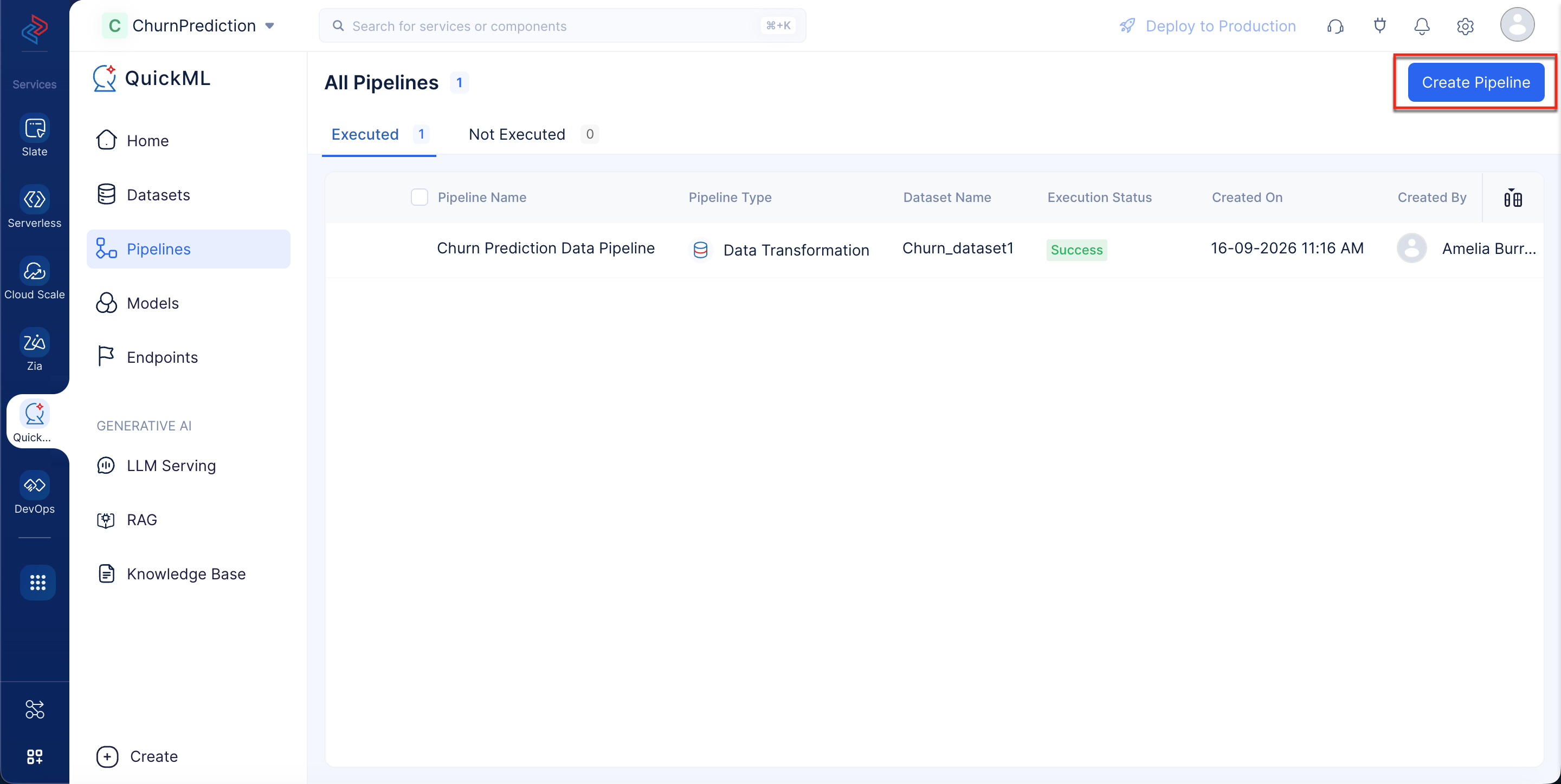
2. In the Create Pipeline pop-up window, choose the Prediction pipeline.

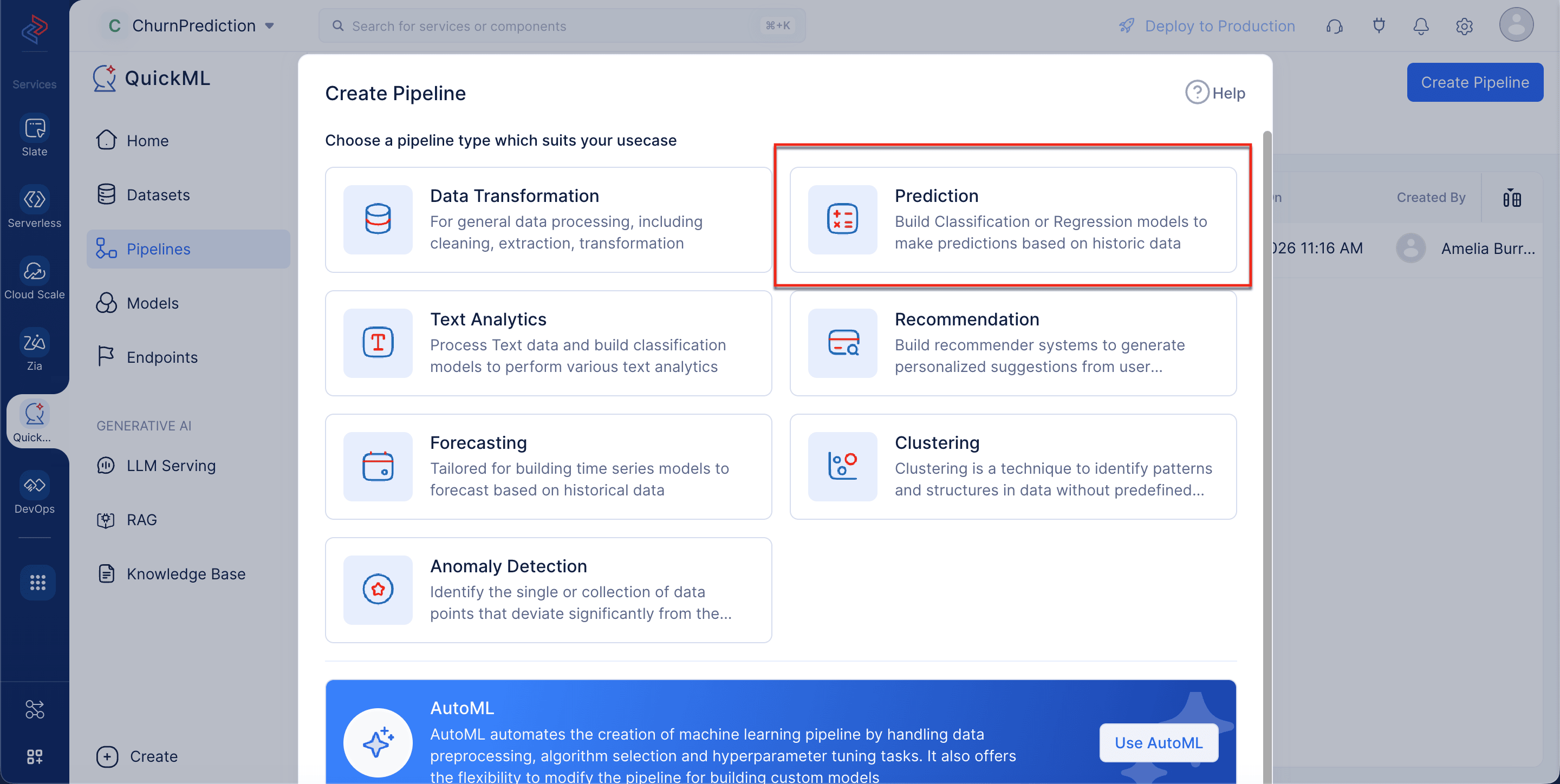
3. Enter the pipeline name as Churn Prediction, choose Churn_datatset1, and churn_risk_score as the target column. Then click Create.

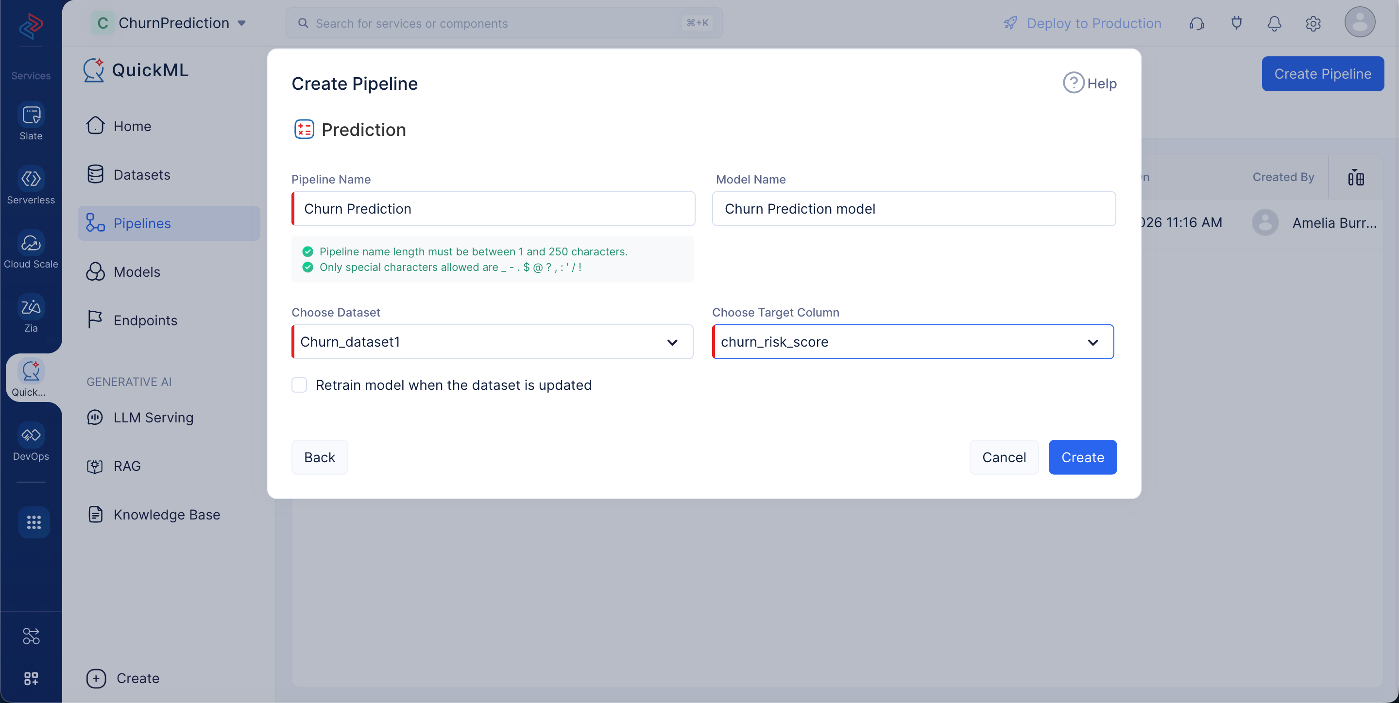
Model creation

The next step is to create the model in the pipeline editor. First select the appropriate encoders to convert categorical or non-numeric data into a numerical format that machine learning algorithms can work with effectively.

Stage 1: Ordinal encoding

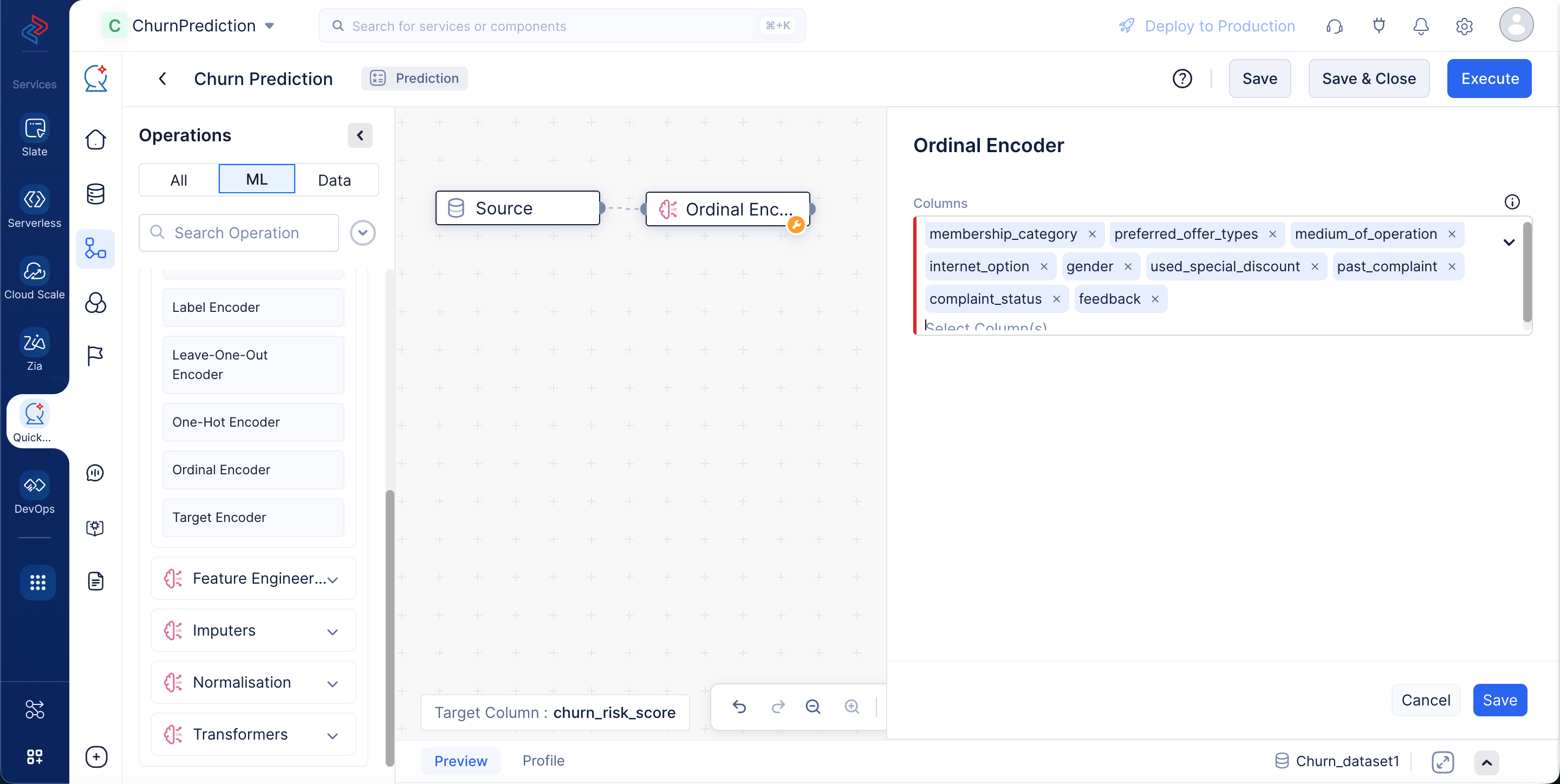
Here, we’re using ordinal encoding to encode “membership_category”, “preferred_offer_types”, “medium_of_operation”, “internet_option”, “gender”, “used_special_discount”, “past_complaints”, “complaint_status” and “feedback”. It assigns integers to the categories based on their order, making it possible for machine-learning algorithms to capture the ordinal nature of the data.

To use the Ordinal Encoder node, navigate to ML tab > ML operations > Encoding component > Ordinal Encoder to turn the selected category columns into numerical columns.

Stage 2: One-hot encoder

One-hot encoding is applied to categorical columns in a dataset, where each category represents a distinct class or group. This increases the dimensionality of the dataset because it creates a new binary column for each unique category. The number of binary columns is equal to the number of unique categories minus one, as you can infer the presence of the last category from the absence of all others.

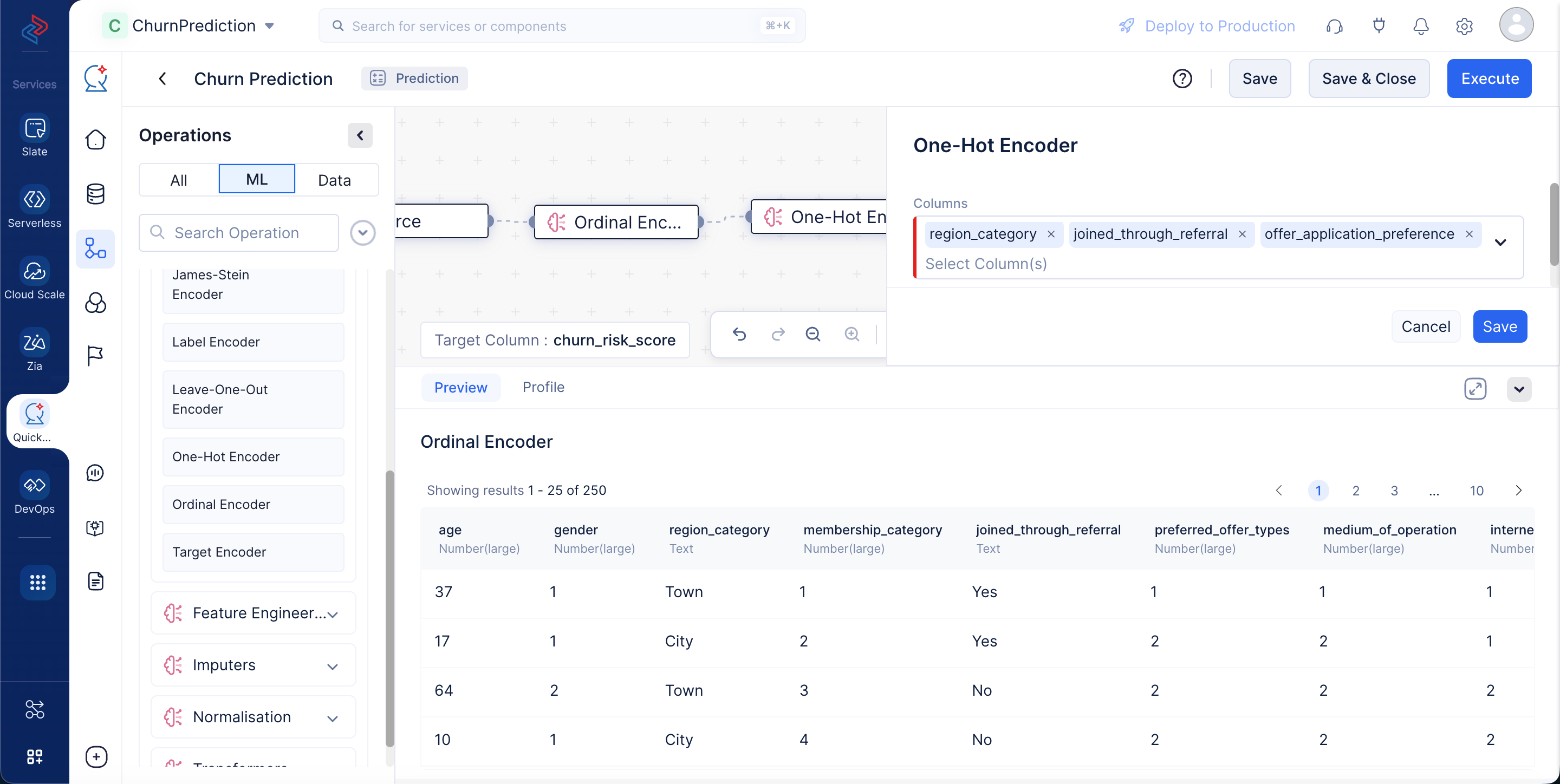
Here, we’re using the One-Hot Encoder node to encode “region_category”, “joined_through_referral” and"offer_application_preference".

To use the One-Hot Encoder node, navigate to ML tab > ML operations > Encoding Component > One-Hot Encoder in QuickML to turn the selected category columns into numerical columns.

Stage 3: Feature selection

Feature selection is the process of selecting the most relevant and important features (variables or columns) from a dataset to use for model training and analysis. The main goal is to enhance the performance, efficiency, and interpretability of machine-learning models. This process is especially important when working with high-dimensional datasets because it helps reduce over-fitting, decrease computation time, and improve model clarity.

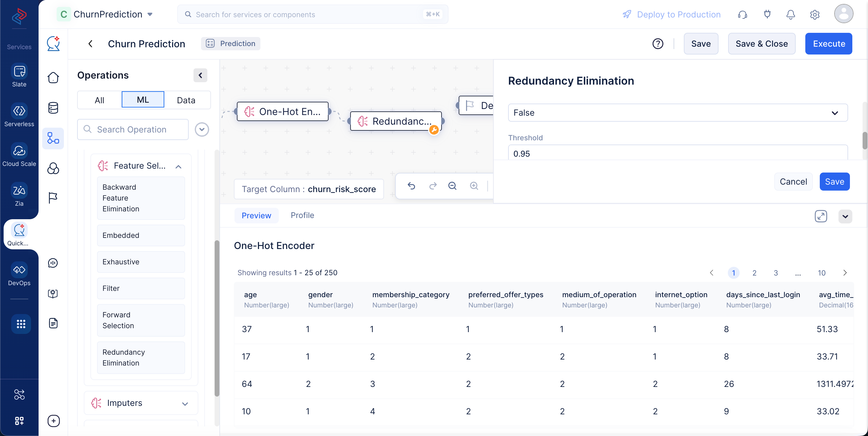
In this case, we’re using the Redundancy Elimination feature selection technique to select the features. This method identifies and removes redundant features—those that provide duplicate or highly correlated information and do not significantly improve model performance. To apply this, navigate to ML tab > ML operations > Feature Engineering component > Feature Selection > Redundancy Elimination.

Stage 4: ML algorithm selection

The next step in ML pipeline building is selecting the appropriate algorithm for training the preprocessed data. Here, we’ll use the XGBoost classification algorithm to train the data.

XGBoost (Extreme Gradient Boosting) is a popular and powerful machine-learning algorithm commonly used for classification tasks. It’s an ensemble learning method that combines the predictions of multiple decision trees to create a strong predictive model. XGBoost is known for its speed, scalability, and ability to handle complex datasets.

We can quickly construct the XGBoost Classification method in QuickML’s ML Pipeline Builder by dragging and dropping the XGBoost Classification node from ML tab > ML operations > Algorithm > Classification > XGBoost Classification.

To make sure the model is optimized for our particular dataset, we may also adjust the tuning parameters; in our case, we can just stick with the default settings. When everything is configured, we may save the pipeline for further testing and deployment.

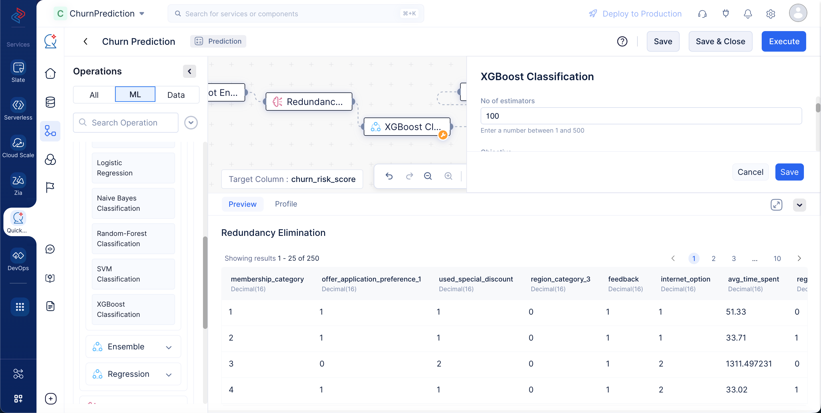
Once we drag and drop the algorithm node, its end node will be automatically connected to the destination node. Click Save to save the pipeline.

Execute the pipeline by clicking the Execute button at the top-right corner of the pipeline builder page.

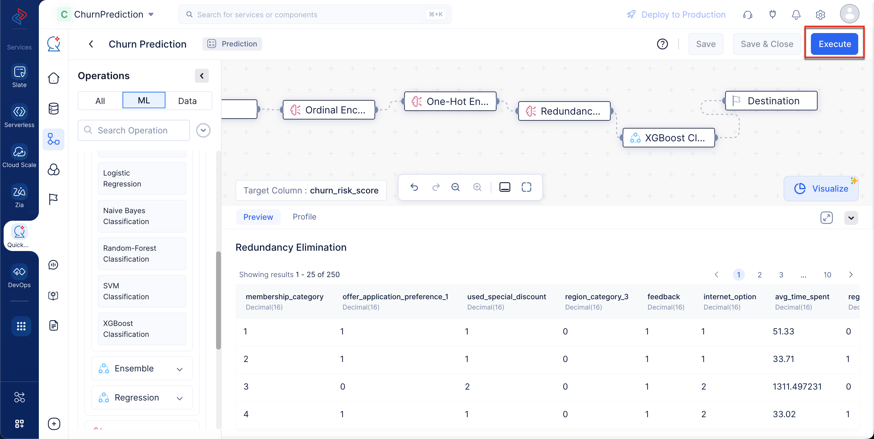
This will redirect you to the executed pipeline page with execution status.

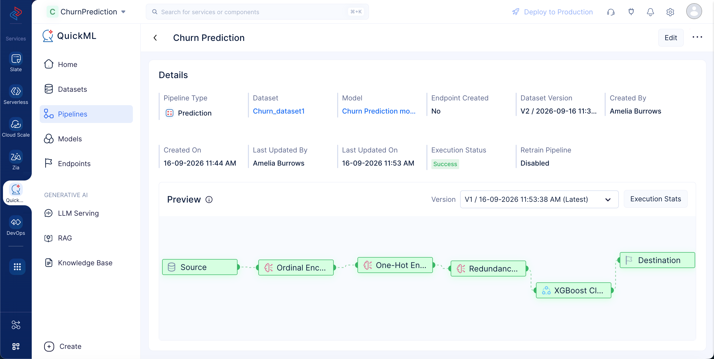
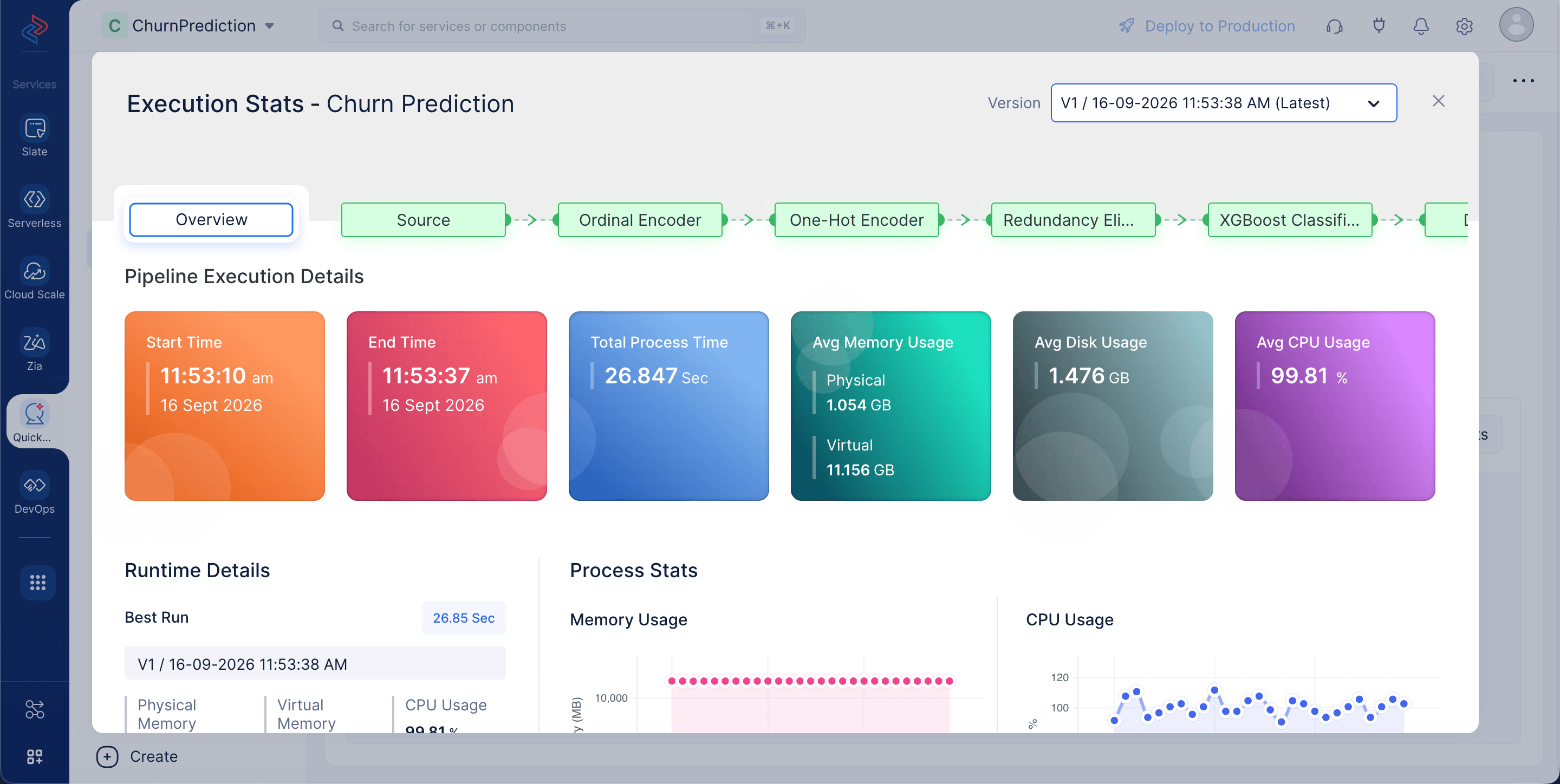
Click Execution Stats to view compute details about each stage of the model execution.

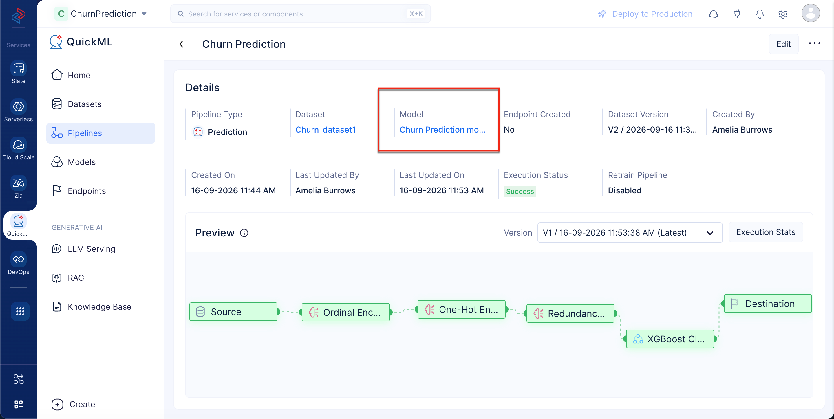
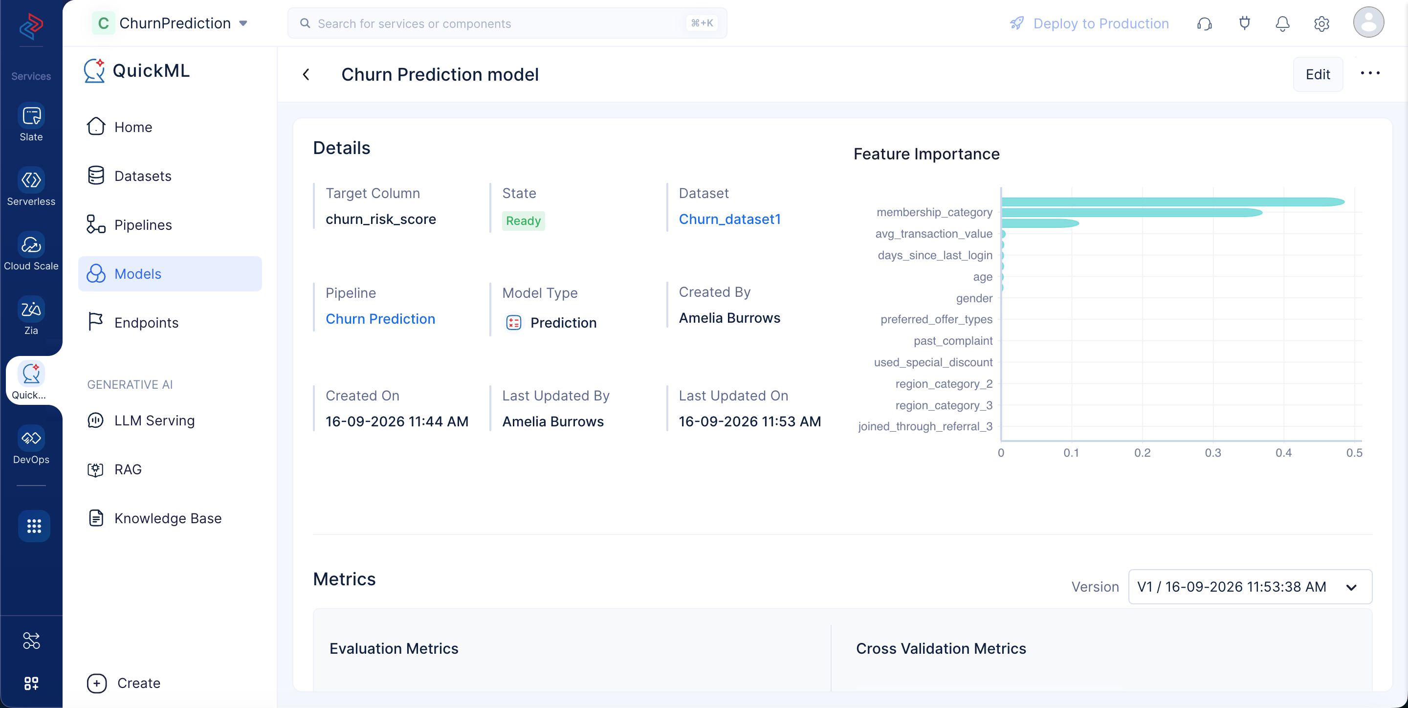
The prediction model is created and can be examined under the Model section (click on Churn Prediction model) following the successful completion of the ML workflow.

This offers valuable insights into the model’s efficiency and performance when making predictions based on the data.