Time Series Algorithms

Time series forecasting is a predictive analytics task that involves the predicting future data points by utilizing the historical data collected over time. Let’s deep dive into how forecasting in time series works and explore different algorithms that are being used to generate forecasting models.

Forecasting

Forecasting involves using statistical methods to predict future values by examining the trends and patterns in past data. This analysis helps business owners make well-informed decisions about future course of actions based on the predictions generated by the model.

Time series forecasting algorithms can be classified into two categories: univariate and multivariate, each leading to the creation of corresponding types of models.

1. Univariate Forecasting

Univariate forecasting models are built using univariate datasets, which contain only a single feature or variable that is recorded over time. These models focus exclusively on the temporal patterns, trends, and seasonality of that one variable for future forecasts, without incorporating the influence of other factors.

Algorithmsused to build the univariate forecasting models include:

• Moving Average - MA
• Exponential Smoothing
• Holt Winter’s Method
• Auto Autoregressive Integrated Moving Average - Auto ARIMA
• Seasonal Autoregressive Integrated Moving Average - SARIMA
• Autoregressive Moving Average - ARMA
• Auto Regressor Let’s understand how each of the algorithms works in detail.

a. Moving Average

The Moving Average (MA) model is a commonly used statistical technique for forecasting in time series analysis. Instead of calculating the average of past data points, it predicts future values based on a linear combination of past forecast errors (or residuals) over a fixed number of periods, known as the “window size.” This method smooths out random fluctuations, making it helpful for identifying short-term trends and patterns in the data.

While the MA model is easy to apply and can be useful for various types of time series data, it relies solely on past errors and does not directly account for past values or other external factors that may affect the data. As a result, it is often recommended to combine the Moving Average model with other forecasting methods, like AutoRegressive models, to improve accuracy and capture more complex dynamics in the data.

The number of past forecast errors used in a Moving Average (MA) model is defined by the MA order or lag (q). The MA order indicates how many previous error terms (lags of the residuals) are included in the model to predict the current value.

For example, in an MA(q) model:

• If q = 1, the model uses the previous error term (the first lag of the residual).
• If q = 2, it uses the previous two error terms (the first and second lags), and so on. The choice of the MA order can significantly impact the model’s performance.

Advantages

• This Moving Average algorithm is well-suited for short-term forecasting, such as predicting sales for the next few periods.
• It can help remove noise from time series data, making it easier to identify underlying patterns or trends by smoothing out random fluctuations.

Disadvantages

• Moving Average (MA) model is not suitable for long-term forecasting as it only relies on past forecast residuals(errors) and does not directly account for past values or other external factors that may affect the data in the long run.
• It may react slowly to sudden changes or trends in the data based on the window size of residuals used for predictions.
• MA models are primarily used for univariate time series forecasting, where the focus is on a single variable over time and its past errors. However, in multivariate time series forecasting, where multiple variables are involved, moving averages do not perform well.
• In multivariate time series analysis, the goal is often to understand the relationships between multiple variables and to leverage these correlations for better forecasting.
• The direct application of a simple moving average model to individual variables independently in a multivariate data fails to capture the potential interdependencies between the variables.

b. Auto Regressive Model

AutoRegressive (AR) models are a class of statistical models commonly used in time series analysis to forecast future values by using past values in the time series as input. They are particularly useful for capturing temporal dependencies in the data by assessing the correlation between preceding and succeeding values in the series. The model predicts future values as a linear combination of past observations, relying on the assumption that past values have a direct influence on future behavior.

AR order (p), can be defined as the number of past observations used in an AutoRegressive (AR) model. It indicates how many previous values (lags) of the time series are included in the model to predict the current value.

For example, in an AR(p) model:

• If p = 1, the model uses the previous value (the first lag).
• If p = 2, it uses the previous two values (the first and second lags), and so on. The choice of the AR order can significantly impact the model’s performance.

Advantages

• AR models are effective in capturing the temporal dependencies present in time series data. By regressing the current value on its own past values, they can capture patterns and trends in the data.
• The parameters of AR models have clear interpretations. Each autoregressive parameter represents the influence of a specific lagged value on the current value, making it easy to understand the relationship between past and present observations.
• AR models are robust to outliers and handle noisy data well. They can effectively filter out short-term fluctuations and focus on capturing long-term trends in the data.
• AR models are computationally efficient, particularly for small to moderate-sized datasets. They require relatively fewer parameters compared to other time series models, making them suitable for quick analysis and forecasting.

Disadvantages

• AR models assume a linear relationship between past and present observations. This assumption may not hold for all time series data, particularly for non-linear relationships or complex patterns.
• AR models assume that the underlying time series is stationary, meaning that its statistical properties do not change over time. However, many real-world time series exhibit non-stationary behavior, which can limit the applicability of AR models.
• Choosing the appropriate order (AR lag(p)) for the AR model can be challenging and may require iterative experimentation or statistical diagnostics. Selecting an incorrect order can lead to poor model performance and inaccurate forecasts.
• AR models may struggle to provide accurate forecasts for long-term horizons, especially when the underlying data is highly volatile or subject to structural changes.

c. ARMA Model

ARMA (AutoRegressive Moving Average) is a time series forecasting method that combines both AutoRegressive and Moving Average components. It builds a statistical model by using the past values from AutoRegressive and past residuals(errors) from Moving Average methods to predict future values. This model is particularly used in capturing short-term dependencies and patterns in stationary time series data.

• Autoregressive (AR) Component: In the autoregressive component, the current value of the time series is modelled as a linear combination of its previous values. The “auto” in autoregressive signifies that the current value is regressed on its own past values. Higher values of p capture more complex dependencies.
• Moving Average (MA) Component: In the moving average component, the current value of the time series is modelled as a linear combination of past forecast errors.The moving average parameters determine the weights assigned to past forecast errors in predicting the current value. Similar to autoregressive models, higher values of q capture more complex dependencies.

ARMA models combine both autoregressive and moving average components to capture the temporal dependencies and random fluctuations present in the data.

An ARMA(p, q) model is represented as the sum of the AR (p) and MA (q) components.

Advantages

• ARMA models can capture a wide range of patterns and dynamics present in time series data, making them versatile for various applications.
• The parameters of ARMA models have clear interpretations, allowing analysts to understand the underlying relationships between past observations and future predictions.
• ARMA models are robust to outliers and can handle noisy data well, making them suitable for real-world datasets with irregularities.
• ARMA models are computationally efficient, particularly for small to moderate-sized datasets, allowing for quick model estimation and forecasting.

Disadvantages

• ARMA models assume that the underlying time series is stationary, meaning that its statistical properties do not change over time. However, many real-world time series exhibit non-stationary behavior, which can limit the applicability of ARMA models.
• ARMA models may struggle to provide accurate forecasts for long-term horizons, especially when the underlying data is highly volatile or subject to structural changes.
• Choosing the appropriate order (p and q) for the AR and MA components of an ARMA model can be challenging and may require iterative experimentation or statistical diagnostics.
• The performance of ARMA models can be sensitive to the initial parameter estimates, leading to potential convergence issues or suboptimal solutions, particularly in high-dimensional parameter spaces.

d. ARIMA Model

The ARIMA (AutoRegressive Integrated Moving Average) model is a popular statistical method designed for time series forecasting to handle non-stationary data by incorporating differencing component in addition to AR and MA components as in ARMA model. It is a versatile and powerful method, as it can be applied to both stationary and non-stationary time series data.

Here’s a breakdown of its components:

• AutoRegressive (AR) term: Represents the relationship between an observation and a certain number of lagged observations (previous time steps). In an AR (p) model, the value of the series at time ’t’ depends linearly on the values at times ’t-1’, ’t-2’, …, ’t-p'.
• Integrated (I) term: Refers to the differencing of raw observations to make the time series stationary. Stationarity implies that the statistical properties of a time series, such as mean and variance, do not change over time. The order of differencing, denoted as ’d’, indicates how many differences are required to achieve stationarity.
• Moving Average (MA) term: Accounts for the relationship between an observation and a residual error from a moving average model applied to lagged observations. In an MA(q) model, the value of the series at time ’t’ depends linearly on the error terms at times ’t-1’, ’t-2’, …, ’t-q'.

The ARIMA model is denoted as ARIMA(p, d, q), where:

• ‘p’ is the order of the autoregressive part.
• ’d’ is the degree of differencing.
• ‘q’ is the order of the moving average part. The ARIMA model makes predictions based on the linear combination of past observations, differencing to stabilise the series, and an error term that captures unexpected fluctuations not explained by the model.

Auto ARIMA

Auto ARIMA automatically searches through a range of possible ARIMA models, including different combinations of autoregressive (AR), integrated (I), and moving average (MA) components, to identify the model that best fits the data. It evaluates each model based on statistical criteria such as AIC (Akaike Information Criterion) or BIC (Bayesian Information Criterion) to determine the optimal model.

Advantages

• ARIMA can handle a wide range of time series data, including economic, financial, and social data, making it applicable in various fields.
• The model parameters (p, d, q) can provide insights into the underlying dynamics of the time series, such as the lag effect and the impact of differencing.
• ARIMA is based on solid statistical principles, making it a reliable method for time series analysis.
• ARIMA can generate forecasts for future time periods, providing valuable insights for decision-making and planning.
• ARIMA models do not require additional external factors or covariates, making them relatively straightforward to implement and interpret.

Disadvantages

• ARIMA assumes that the time series is stationary or can be made stationary through differencing. In practice, achieving stationarity can be challenging for some datasets.
• Traditional ARIMA models are not well-suited for capturing seasonal patterns in the data. Seasonal ARIMA (SARIMA) or other methods are needed for seasonal data.
• They are linear and may not effectively capture complex non-linear relationships present in some time series data.
• ARIMA models require a sufficient amount of historical data to estimate the model parameters accurately. In cases of short or sparse data, ARIMA may not perform well.
• ARIMA assumes that observations are independent of each other, which may not hold true for all time series data, particularly in cases of autocorrelation or serial correlation.

e. SARIMA Model

Seasonal Autoregressive Integrated Moving Average (SARIMA) is an extension of the ARIMA model that incorporates seasonality into the analysis and forecasting of time series data. SARIMA models are particularly useful for data that exhibit both non-seasonal and seasonal patterns:

• Seasonal Differencing: SARIMA involves differencing the time series not only to remove trends but also to remove seasonal patterns. This is done by subtracting the observation at time ’t’ from the observation at time ’t-s’, where ’s’ represents the seasonal period.
• Seasonal Autoregressive (SAR) Term: Seasonal AR lag, component accounts for the relationship between the current observation and past observations at seasonal intervals. It captures the seasonal patterns in the data.
• Seasonal Moving Average (SMA) Term: Seasonal MA lag component models the dependence between the current observation and past forecast errors at seasonal intervals.
• Integration: Like in ARIMA, integration is used to make the time series stationary by differencing. The order of integration (denoted by ’d’) represents the number of non-seasonal differences needed to achieve stationarity.
• Autoregressive (AR) and Moving Average (MA) Terms: These components, similar to ARIMA, capture the non-seasonal dynamics of the time series.

Advantages

• SARIMA explicitly models seasonal patterns in the data, allowing for more accurate forecasts of time series with periodic fluctuations, such as monthly sales data or quarterly economic indicators.
• SARIMA models can handle a wide range of seasonal patterns, including multiplicative and additive seasonality, as well as irregular seasonal patterns.
• Like ARIMA, SARIMA models provide interpretable parameters (e.g., AR, MA, seasonal AR, seasonal MA) that can offer insights into the underlying dynamics of the time series.
• SARIMA models can be robust to changes in the underlying data patterns, provided that the appropriate seasonal period and model parameters are selected.

Disadvantages

• SARIMA models are more complex than non-seasonal ARIMA models, requiring additional parameters to capture seasonal dynamics. This complexity can make model estimation and interpretation more challenging.
• Selecting the appropriate seasonal period and determining the orders of the AR, MA, seasonal AR, and seasonal MA terms can be difficult and may require extensive model diagnostics and testing.
• Estimating SARIMA models, especially for large datasets or models with many parameters, can be computationally intensive and time-consuming.
• SARIMA assumes that the time series is stationary after differencing. Ensuring stationarity may require careful examination of the data and iterative model fitting.

Despite these challenges, SARIMA remains a powerful tool for time series forecasting, for data that exhibit both non-seasonal and seasonal patterns. With careful model specification and parameter selection, SARIMA models can provide accurate forecasts and valuable insights into time series data.

f. Exponential Smoothing Model

Exponential smoothing is a time series forecasting method for univariate data that can be extended to support data with a systematic trend or seasonal component.

It also make predictions based on past observations like ARIMA but with a key difference in how they weigh these observations:

• Exponentially Decreasing Weights
  • Unlike ARIMA, where weights can be arbitrary, Exponential Smoothing assigns exponentially decreasing weights to past observations. This means recent observations have a much greater influence on the forecast than older ones.
  • Example: If you’re predicting today’s sales, yesterday’s sales will have a bigger impact on the forecast than sales from a week ago.
• Types of Exponential Smoothing
  • Simple Exponential Smoothing (SES): Suitable for data without a trend or seasonality. It only uses past observations.
  • Holt’s Linear Trend Model: Extends SES to capture trends in the data.
  • Holt-Winters Seasonal Model: Further extends to capture seasonality (repeating patterns like monthly sales peaks).

Advantages

• Handles different patterns implies that it can be adapted to handle different types of time series data, including those with:
  • No trend (Simple Exponential Smoothing)
  • Linear trends (Holt’s Linear Trend Model), and
  • Seasonal patterns (Holt-Winters Seasonal Model)
• Requires relatively less historical data compared to some other more complex forecasting methods like ARIMA or machine learning models.
• Responsive to Changes because recent observations are given more weight, the method can quickly adapt to changes or shifts in the data

Disadvantages

• Exponential smoothing may struggle to capture complex relationships or irregular fluctuations present in the data.
• The performance of exponential smoothing models can be sensitive to the choice of smoothing parameters, such as the smoothing factor (alpha).
• Exponential smoothing assumes that the underlying time series is stationary, meaning that its statistical properties remain constant over time. However, many real-world time series exhibit non-stationary behavior.
• Exponential smoothing models are sensitive to outliers or extreme values in the data.

g. Holt Winter’s Seasonal Model

Holt-Winters’ method, also known as triple exponential smoothing, is a widely used technique for forecasting time series data, especially when dealing with data that exhibit trend and seasonality. It extends simple exponential smoothing to handle these components more effectively.

• Level Component (lt): It represents the average value of the series over time. It is updated at each time step based on the observed value and the previous level.The updated level at time ’t’ is a combination of the observed value ‘yt’, the previous level ’lt-1’, and the previous trend ‘bt-1’. It’s calculated using a smoothing parameter alpha.
• Trend Component (bt): It captures the direction and rate of change in the series over time. It is updated to reflect the trend observed in recent data.The updated trend at time ’t’ is a combination of the difference between the current level and the previous level, and the previous trend. It’s calculated using a smoothing parameter beta.
• Seasonal Component (st): It accounts for seasonal variations or patterns that repeat at fixed intervals (e.g., daily, weekly, monthly). It’s updated to reflect the seasonal behaviour observed in the data. The updated seasonal component at time ’t’ is a combination of the observed value and the corresponding seasonal component observed at the same time in previous seasons. It’s calculated using a smoothing parameter gamma.

There are two main types of Holt-Winters models

Additive model: The Additive model is used when the seasonal variations are roughly constant through the series. It is suitable when the magnitude of the seasonal effect does not depend on the level of the time series.

Level :	  Lt=α(Yt−St−m)+(1−α)(Lt−1+Tt−1)
Trend:	  Tt=β(Lt−Lt−1)+(1−β)Tt−1
Season:	  St=γ(Yt−Lt)+(1−γ)St−m
Forecast: Yt+h=L t+hTt+St−m+h	

Multiplicative Model: Multiplicative model is used when the seasonal variations change proportionally with the level of the series. It is suitable when the magnitude of the seasonal effect varies with the level of the time series.

Level :	  Lt=α(Yt/St−m)+(1−α)(Lt−1+Tt−1)
Trend:	  Tt=β(Lt−Lt−1)+(1−β)Tt−1
Season:	  St=γ(Yt/Lt)+(1−γ)St−m
Forecast: Yt+h=(Lt+hTt)St−m+h

Advantages

• It’s specifically designed to capture and forecast time series data with both trend and seasonality, making it suitable for a wide range of real-world applications.
• The method adapts to changes in the underlying data patterns over time, making it robust in dynamic environments where the data may exhibit evolving trends or seasonal patterns.
• The resulting forecasts can be easily interpreted as they are based on the level, trend, and seasonal components, providing insights into the future behavior of the time series.
• While the method involves multiple components and parameters, it’s relatively straightforward to implement compared to more complex forecasting techniques.

Disadvantages

• Selecting appropriate values for the smoothing parameters alpha, beta, and gamma can be challenging and may require expertise or extensive experimentation, especially for datasets with varying characteristics.
• Sensitive to outliers or sudden changes in the data, which can impact the accuracy of forecasts, particularly if these anomalies are not appropriately addressed.
• Like other exponential smoothing methods, Holt-Winters’ method assumes linear relationships between the components, which may not adequately capture complex non-linear patterns present in some time series data.
• Estimating and updating the components of the Holt-Winters’ method for large datasets or high-frequency data can be computationally intensive, especially if implemented without optimization techniques

2. Multivariate Forecasting Algorithms

a. Vector Auto Regressor (VAR)

The Vector Auto Regression (VAR) model is a multivariate time series algorithm used to capture the linear interdependencies among multiple time series. It generalizes the univariate autoregressive (AR) model to multivariate time series data. Each variable in a VAR model is a linear function of past lags of itself and past lags of all the other variables in the system.

Advantages

• VAR models are well-suited for capturing the dynamic relationships between multiple time series without requiring the specification of dependent and independent variables. This makes them flexible in modelling complex interdependencies among variables.
• All variables in a VAR model are treated as endogenous, meaning there is no need to categorise them as dependent or independent. This symmetry allows for a more comprehensive understanding of how the variables interact with each other over time.
• VAR models explicitly account for the lagged effects of each variable on itself and others, allowing for a detailed analysis of temporal dependencies.
• The VAR framework allows for Granger causality testing, which can identify whether one time series can predict another, providing insights into causal relationships between variables.
• VAR models facilitate impulse response analysis, which helps to understand the effect of a shock to one variable on the other variables in the system over time. This is particularly useful in policy analysis and economic forecasting.

Disadvantages

• VAR models require the estimation of a large number of parameters, especially when dealing with many variables and lags. This can lead to over fitting, making the model sensitive to noise and reducing its generalizability.
• The large number of parameters to estimate means that VAR models require a significant amount of data to achieve stable and reliable results. This can be a limitation when working with short time series or sparse data.
• Although VAR models are powerful, interpreting the relationships between variables can be challenging, especially when the model includes many variables and lags. The model’s output can be complex and may require advanced statistical knowledge to interpret correctly.
• VAR models assume linear relationships between variables. In reality, relationships between time series variables can be non-linear, which may limit the model’s effectiveness in capturing the true dynamics.
• The choice of lag length p is crucial in VAR modelling. Too few lags can lead to model misspecification, while too many can cause overfitting. Selecting the optimal lag length is not always straightforward and often requires careful testing and validation.
• Unlike Structural VAR (SVAR) models, standard VAR models do not provide a structural interpretation of the relationships between variables. This can be a limitation in economic and policy analysis, where understanding the underlying mechanisms is important.
• When the variables in the VAR model are highly correlated, multicollinearity can become a problem, leading to unreliable estimates of the coefficients. This can make it difficult to discern the true impact of each variable on others.
• As the number of variables and lags increases, the computational burden of estimating the model parameters grows. This can make VAR models computationally intensive, especially for large datasets.

Cross Validation

Cross-validation in time series is a technique used to evaluate the performance of a model on a time series dataset. Unlike typical k-fold cross-validation used in standard machine learning, time series data has a temporal order that must be preserved. Therefore, specific methods are used to handle this temporal dependency.

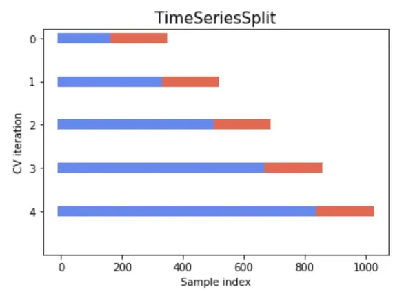
i. Rolling Time Series Split

• This method involves splitting the time series data into training and validation sets multiple times in such a way that the training set always precedes the validation set.
• It simulates the way new data becomes available over time and ensures that the model is always tested on future data, relative to the training set.
• Refer to the below image for data split understanding

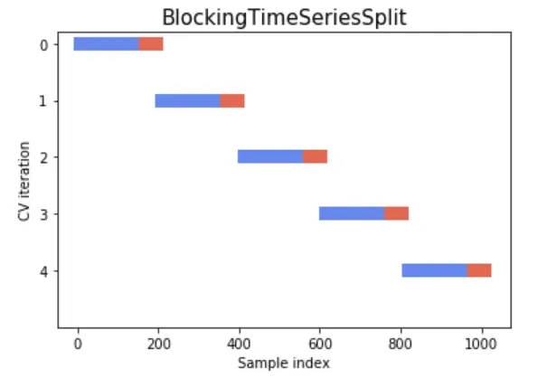
ii. Blocking Time Series Split

• Involves splitting the data into contiguous blocks or folds, while ensuring that there is no overlap between the training and testing sets and maintaining the temporal order of the data.
• Prevents the model from seeing future data during training, leading to over fitting.
• Ensures that the training set always precedes the validation set, respecting the time order.

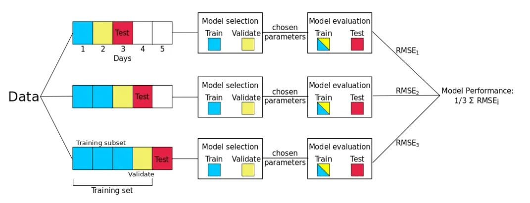
iii. Day Forward Chaining

• Day Forward-Chaining is based on a method called forward-chaining and rolling-origin-recalibration evaluation. Using this method, we successively consider each day as the test set and assign all previous data into the training set
• This method produces many different train/test splits. The error on each split is averaged in order to compute a robust estimate of the model error.

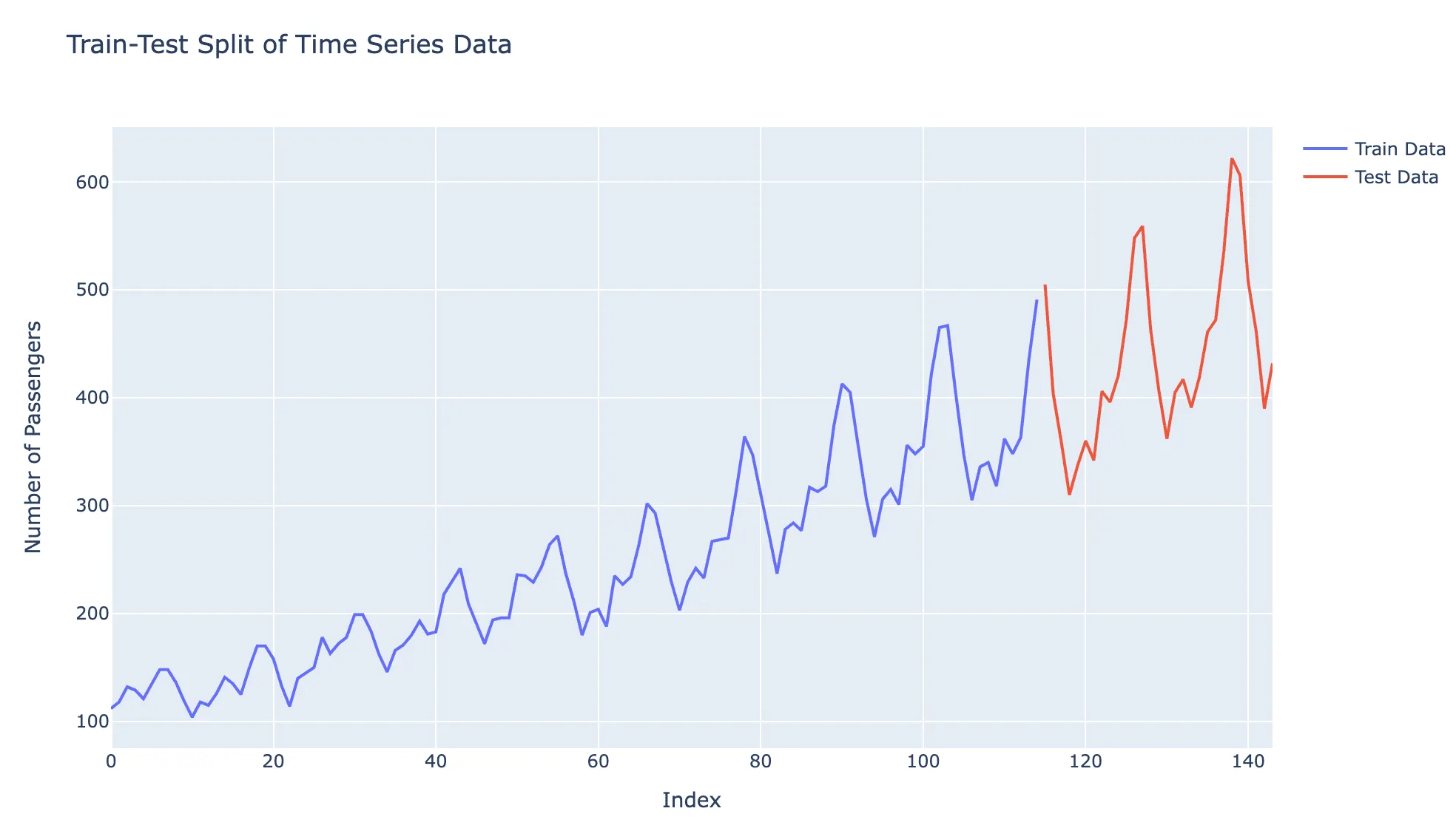
iv. Regular Train Test Split - Default In a standard train-test split scenario, a time series dataset is split into two subsets: a training set and a test set. The training set is used to train the model, which contains historical data, and then tested on the test set, which includes future unseen data. This allows for evaluating the model’s performance and its generalization capabilities by testing its ability to predict future values based on past data.

Visual representation of the Train-test split of the data as follows:

Build a pipeline

QuickML uses smart mode pipeline builder to create time series models. The Smart Builder provides a prebuilt template for time series models, designed to simplify the model development process from data preprocessing to model selection. With these prebuilt templates, operations are predefined, and users are presented with various parameters to configure each stage. This template removes the ambiguity of which stage to use to build a time series model and streamlines the model-building process.

Visualizations

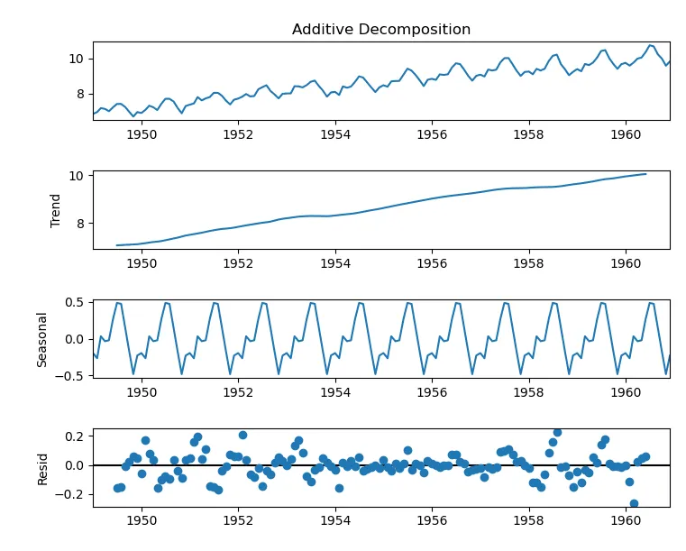
Decomposition Chart

A decomposition chart breaks down time series data into its key components: trend, seasonal, and residual (or noise). It helps validate the presence of these components and understand their contributions to the overall pattern of the data. Decomposition is particularly useful for analyzing time series data recorded at regular intervals over different periods.

In QuickML, the decomposition chart uses the additive technique, where the original time series is represented as the sum of its components:

Original Series = Trend + Seasonality + Residual

This technique assumes that the magnitude of the seasonal and residual variations remains constant across the series.