Anomaly Detection Algorithms
Anomaly detection is an unsupervised machine learning technique that focuses on identifying data points, events, or observations that deviate significantly from the majority of the data. These outliers can represent critical incidents such as fraud, network intrusions, equipment failures, or data quality issues. Instead of predicting predefined labels, anomaly detection models learn normal behavior within the data and flag deviations that may require attention.
Anomaly detection in Catalyst QuickML is broadly categorized into Time Series and Non-Time Series, each offering its own set of algorithms and configurable parameters.
Within Catalyst QuickML, anomaly detection for time series data focuses on identifying abnormal patterns or deviations in sequential data points over time. These methods account for temporal dependencies and seasonality, enabling the detection of sudden spikes, drops, or trend changes.
Before exploring the individual time-series anomaly detection algorithms, it’s important to understand the common parameters used for Anomaly Sensitivity Control, as shown in the image below. These parameters are consistent across all time-series anomaly detection algorithms in Catalyst QuickML and are essential for controlling how anomalies are detected and interpreted. They allow users to fine-tune the threshold, window size, and anomaly scoring method, ensuring that the system accurately differentiates between normal fluctuations and true anomalous behavior.
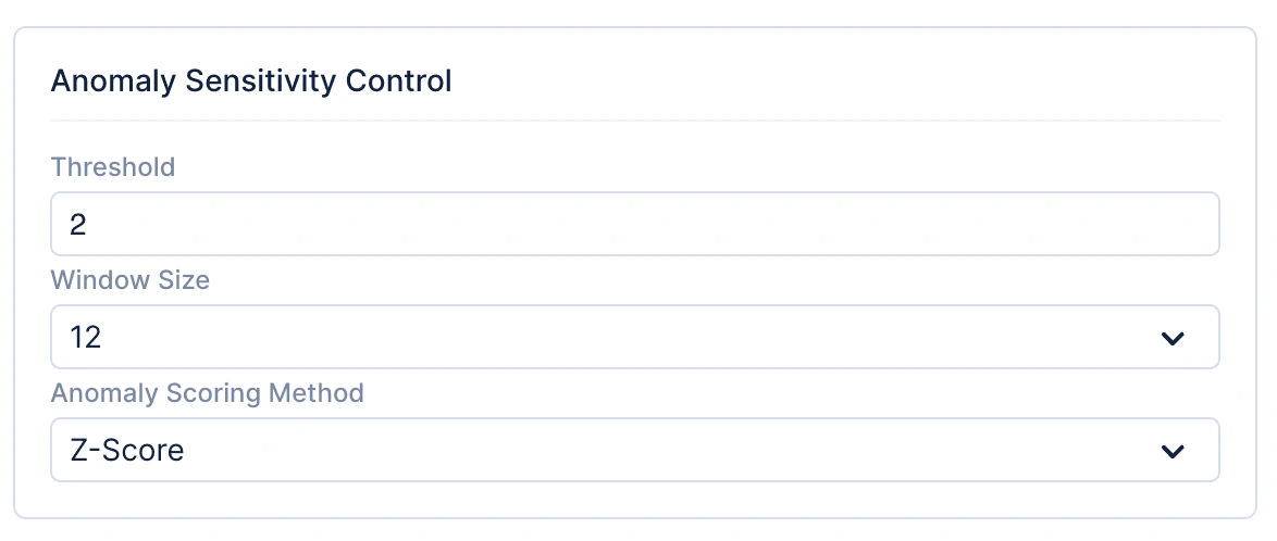
Common parameters:
-
Threshold: Determines how sensitive the model is to deviations from expected behavior. A lower threshold increases sensitivity, flagging smaller fluctuations as anomalies, while a higher threshold reduces false positives.
-
Window size: Defines the rolling window of data points used for analysis. Applicable up to a maximum of 24 time steps.
-
Anomaly scoring method: Currently supports Z-Score, which measures how far a point deviates from the mean in terms of standard deviations.
Below are the time series anomaly detection algorithms supported in Catalyst QuickML, along with their explanations, real-world use cases, and key parameters.
Auto Regressor
Explanation: The Auto Regressor (AR) model predicts future values based on a linear combination of past observations. It assumes that past behavior directly influences the present, with coefficients representing the relationship strength between past and current values. QuickML extends this with flexible regression backends, including Linear Regressor, Random Forest Regressor, AdaBoost Regressor, and Gradient Boosting Regressor, enabling both linear and non-linear temporal modeling.
Mathematical intuition:
Yₜ = c + ∑ᵢ₌₁ᵖ φᵢ Yₜ₋ᵢ + εₜ Where:
- Yt = current value
- c = intercept (constant term)
- ϕi = autoregressive coefficients
- Yt−i = lagged observations
- εt = random noise
Use case: Used in financial forecasting, sensor drift detection, and predictive process monitoring, where recent history significantly affects the next outcome — e.g., predicting short-term stock trends or detecting abnormal fluctuations in temperature sensors.
Key parameters:
| Parameter | Description | Data Type | Possible Values | Default Value |
|---|---|---|---|---|
| select_model_to_fit | Chooses the regression model for fitting time series. | string | {‘Linear Regressor’, ‘Random-Forest Regressor’, ‘AdaBoost Regressor’, ‘Gradient Boosting Regressor’} | ‘Linear Regressor’ |
| max_lag | Defines how many past time steps are used to predict the current value. | int | [1, ∞) | 1 |
Moving Average (MA)
Explanation: The Moving Average model focuses on modeling noise or random shocks within a time series. Instead of using past values directly, it predicts current observations as a weighted sum of past forecast errors. This approach helps smooth short-term volatility and is ideal for detecting unusual deviations from expected residual patterns.
Mathematical intuition:
Yₜ = μ + ∑ᵢ₌₁ᵠ θᵢ εₜ₋ᵢ + εₜ Where:
- Yt = current observation
- μ = mean of the series
- θi = moving average coefficients
- εt−i = past forecast errors
Use case: Applied in stock price anomaly detection, manufacturing output monitoring, and short-term demand forecasting, where identifying irregular error patterns helps uncover transient anomalies or process instability.
Key parameters:
| Parameter | Description | Data Type | Possible Values | Default Value |
|---|---|---|---|---|
| ma_lag (q) | Specifies the number of past forecast errors used to predict future values. | int | [0, 5] | 1 |
ARIMA (AutoRegressive Integrated Moving Average)
Explanation: ARIMA integrates three components:
- AR (AutoRegressive) – Uses past values
- I (Integrated) – Removes trend and non-stationarity through differencing
- MA (Moving Average) – Models residual noise
By combining these, ARIMA captures both temporal dependence and trend shifts. It’s highly effective for stationary time series and detecting deviations that violate established statistical relationships over time.
Mathematical intuition:
Y′ₜ = c + ∑ᵢ₌₁ᵖ φᵢ Y′ₜ₋ᵢ + ∑ⱼ₌₁ᵠ θⱼ εₜ₋ⱼ + εₜ Where Yt′ is the differenced series after applying order d.
Use case: Widely used in economic indicator monitoring, system log anomaly detection, and production line forecasting, where detecting shifts from long-term trends or cyclical stability is crucial.
Key parameters:
| Parameter | Description | Data Type | Possible Values | Default Value |
|---|---|---|---|---|
| ar_lag (p) | Number of lag observations included in the model. | int | [0, 5] | 1 |
| ma_lag (q) | Number of lagged forecast errors in the prediction equation. | int | [0, 5] | 1 |
| integration (d) | Number of times the data is differenced to achieve stationarity. | int | [0, 5] | 0 |
ARMA (AutoRegressive Moving Average)
Explanation: ARMA combines the strengths of AR and MA models but assumes the series is stationary (no differencing). It captures both dependency on past observations and correlations in error terms, providing a balance between trend sensitivity and noise filtering.
Mathematical intuition:
Yₜ = c + ∑ᵢ₌₁ᵖ φᵢ Yₜ₋ᵢ + ∑ⱼ₌₁ᵠ θⱼ εₜ₋ⱼ + εₜ Use case: Used in network latency monitoring, server performance analysis, and stable process anomaly detection, where consistent behavior over time makes small deviations highly significant.
Key parameters:
| Parameter | Description | Data Type | Possible Values | Default Value |
|---|---|---|---|---|
| ar_lag (p) | Number of lag observations used in the model. | int | [0, 5] | 1 |
| ma_lag (q) | Number of lagged forecast errors in the model. | int | [0, 5] | 1 |
Auto ARIMA
Explanation: Auto ARIMA automates ARIMA model selection by evaluating multiple combinations of parameters (p,d,q) and optionally seasonal parameters based on information criteria (like AIC or BIC). This allows optimal fitting without manual parameter tuning and ensures that the model adapts to changing time dynamics.
Mathematical intuition: Automatically selects parameters minimizing:
AIC = 2k − 2ln(L) Where k = number of parameters and L = maximum likelihood estimate.
Use case: Ideal for seasonal retail forecasting, utility consumption anomaly tracking, and automated operational monitoring, where time series exhibit both periodic and non-periodic irregularities.
Key parameters:
| Parameter | Description | Data Type | Possible Values | Default Value |
|---|---|---|---|---|
| seasonal | Indicates whether the model should account for seasonality. | bool | {True, False} | True |
| ar_lag (p) | Non-seasonal AR lag parameter. | int | [0, 5] | 1 |
| ma_lag (q) | Non-seasonal MA lag parameter. | int | [0, 5] | 1 |
| integration (d) | Non-seasonal differencing order. | int | [0, 5] | 0 |
| periodicity (s) | Seasonal period length (e.g., 12 for monthly data). | int | [0, ∞) | 12 |
| integration (D) | Seasonal differencing order. | int | [0, 5] | 0 |
| max_order | Maximum total order of the model (optional). | int | [0, 5] | 5 |
SARIMA (Seasonal ARIMA)
Explanation: SARIMA extends ARIMA by including seasonal autoregressive, differencing, and moving average components, allowing it to model periodic fluctuations (e.g., daily, monthly, yearly cycles). It excels in detecting anomalies that occur relative to seasonal expectations.
Mathematical intuition:
Φᴾ(Bˢ) φᵖ(B) (1 − B)ᵈ (1 − Bˢ)ᴰ Yₜ = Θᵠ(Bˢ) θᵩ(B) εₜ Where:
- s = seasonal period
- (p,d,q) = non-seasonal parameters
- (P,D,Q) = seasonal parameters
Use case: Applied in energy load anomaly detection, climate monitoring, and sales seasonality analysis, where deviations from expected seasonal behavior signal potential anomalies.
Key parameters:
| Parameter | Description | Data Type | Possible Values | Default Value |
|---|---|---|---|---|
| ar_lag (p) | Non-seasonal AR term. | int | [0, 5] | 1 |
| ma_lag (q) | Non-seasonal MA term. | int | [0, 5] | 1 |
| integration (d) | Non-seasonal differencing. | int | [0, 5] | 0 |
| seasonal_ar (P) | Seasonal AR term. | int | [0, 5] | 1 |
| seasonal_ma (Q) | Seasonal MA term. | int | [0, 5] | 1 |
| seasonal_integration (D) | Seasonal differencing. | int | [0, 5] | 0 |
| periodicity (s) | Seasonal period (e.g., 12 for monthly seasonality). | int | [0, ∞) | 12 |
| enforce_stationarity | Whether to enforce stationarity in the model. | bool | {True, False} | False |
| enforce_invertibility | Whether to enforce invertibility of the model. | bool | {True, False} | False |
Exponential Smoothing
Explanation: Exponential Smoothing predicts future values by giving exponentially decreasing weights to older observations. This emphasizes recent data while maintaining awareness of the overall trend. It’s highly responsive to sudden changes in trend or level.
Mathematical intuition:
Ŷₜ₊₁ = αYₜ + (1 − α)Ŷₜ Where:
- Y^t+1 = forecast
- α = smoothing parameter (0–1)
- Yt = actual value
Use case: Common in inventory control, sales trend monitoring, and machine telemetry, where rapid detection of shifts or decays in recent behavior is vital.
Key parameters:
| Parameter | Description | Data Type | Possible Values | Default Value |
|---|---|---|---|---|
| damped_trends | Whether to apply damping to trend components. | bool | {True, False} | False |
| season | Type of seasonality to apply. | string | {‘Add’, ‘Mul’} | ‘Add’ |
| seasonal_periods | Number of periods in a full seasonal cycle. | int | [1, ∞) | 12 |
Holt-Winter’s Method
Explanation: The Holt-Winter’s method (Triple Exponential Smoothing) extends exponential smoothing by adding trend and seasonal components. It can adapt to level changes, upward or downward trends, and cyclical variations, providing robust anomaly detection for periodic time series.
Mathematical intuition:
Lₜ = α (Yₜ / Sₜ₋ₛ) + (1 − α)(Lₜ₋₁ + Tₜ₋₁)
Tₜ = β (Lₜ − Lₜ₋₁) + (1 − β)Tₜ₋₁
Sₜ = γ (Yₜ / Lₜ) + (1 − γ)Sₜ₋ₛ
Ŷₜ₊ₘ = (Lₜ + mTₜ) Sₜ₋ₛ₊ₘ
Where Lt = level, Tt = trend, St = seasonal component.
Use case: Widely used in retail demand forecasting, resource utilization monitoring, and temperature anomaly detection, where both seasonality and trend shifts must be captured for accurate anomaly identification.
Key parameters:
| Parameter | Description | Data Type | Possible Values | Default Value |
|---|---|---|---|---|
| smoothing_level | Smoothing factor for the level component. | float | [0, 1] | 0.8 |
| smoothing_trend | Smoothing factor for the trend component. | float | [0, 1] | 0.2 |
| damping_trend | Controls the damping of the trend component. | bool | {True, False} | True |
| optimise | Specifies whether parameters should be optimized automatically. | string | {‘Select’, ‘Manual’} | ‘Select’ |
| exponential | Whether to use exponential trend smoothing. | bool | {True, False} | False |
One-Class SVM
Explanation: One-Class SVM (Support Vector Machine) learns a decision boundary around the majority of (normal) data points in feature space. Points that fall outside this boundary are classified as anomalies. It works well in high-dimensional datasets and is effective when anomalies are rare and distinct from normal data.
Mathematical Intuition:
The algorithm finds a function f(x) that is positive for regions with high data density (normal points) and negative for low-density regions (anomalies). It aims to solve:
min (1/2) ||w||² + (1 / (νn)) Σ ξᵢ − ρ
subject to:
(w · φ(xᵢ)) ≥ ρ − ξᵢ , ξᵢ ≥ 0
Where:
- ν: controls the upper bound of outliers
- ξi: slack variables allowing soft margins
- ϕ(x): kernel function mapping data to higher dimensions
Use case: Used in fraud detection, network intrusion detection, or novelty detection in industrial systems where normal behavior is well-defined but anomalies are rare.
Key parameters:
| Parameter | Description | Data Type | Possible Values | Default Value |
|---|---|---|---|---|
| kernel | Specifies the kernel type to use. If none is given, 'rbf' is used. | string | {‘linear’, ‘poly’, ‘rbf’, ‘sigmoid’, ‘precomputed’} | 'rbf' |
| degree | Degree of the polynomial kernel function ('poly'). Ignored by other kernels. | int | [1, ∞) | 3 |
| gamma | Kernel coefficient for 'rbf', 'poly', and 'sigmoid'. | string | {‘scale’, ‘auto’} | 'scale' |
| coef0 | Independent term in kernel function, significant in 'poly' and 'sigmoid'. | float | [0, 1] | 0.0 |
| tol | Tolerance for stopping criterion. | float | [0, 1] | 1e-3 |
| nu | Upper bound on fraction of training errors and lower bound on fraction of support vectors. | float | (0, 1] | 0.5 |
| shrinking | Whether to use the shrinking heuristic. | bool | {False, True} | True |
| max_iter | Hard limit on solver iterations, or -1 for no limit. | int | [1, ∞), {-1} | -1 |
Isolation Forest
Explanation: Isolation Forest identifies anomalies by isolating observations instead of modeling normal data points. It randomly selects a feature and splits the data based on a random threshold. Since anomalies are few and different, they are easier to isolate and require fewer splits. The average path length of trees is shorter for anomalies and longer for normal points.
Mathematical intuition:
The anomaly score is computed as:
s(x, n) = 2^(− E(h(x)) / c(n)) Where:
- E(h(x)): average path length of observation x
- c(n): average path length of unsuccessful search in a Binary Search Tree
- Scores close to 1 → anomalies; near 0.5 → normal
Use case: Commonly used in fraud detection, network intrusion detection, manufacturing defect detection, and IoT sensor anomaly identification. In fraud detection, it helps uncover suspicious transactions that deviate from normal spending behavior. In network intrusion detection, it identifies abnormal access patterns or traffic spikes that may indicate a security breach.
Key parameters:
| Parameter | Description | Data Type | Possible Values | Default Value |
|---|---|---|---|---|
| n_estimators | Number of base estimators (trees) in the ensemble. | int | [1, ∞) | 100 |
| max_samples | Number of samples to draw to train each estimator. | string, int, float | [1, ∞), [0, 1], {'auto'} | 'auto' |
| contamination | Proportion of outliers in the dataset. | string, float | {‘auto’}, (0, 0.5] | 'auto' |
| max_features | Number of features to draw for each estimator. | int, float | [1, ∞), [0, 1] | 1.0 |
| bootstrap | Whether to sample training data with replacement. | bool | {False, True} | False |
Local Outlier Factor (LOF)
Explanation: Local Outlier Factor detects anomalies by comparing the local density of a data point to that of its neighbors. If a point has a substantially lower density than its neighbors, it’s considered an anomaly. LOF is particularly effective in detecting local anomalies rather than global ones.
Mathematical intuition:
LOF is based on the concept of local reachability density (LRD). The LOF score of a data point A is given by:
LOFₖ(A) = ( Σ_{B ∈ Nₖ(A)} [LRDₖ(B) / LRDₖ(A)] ) / |Nₖ(A)| Where:
- Nk(A): k-nearest neighbors of A
- LRDk(A): local reachability density of A
- Values ≈ 1 → normal, > 1 → outlier
Use case: It is effectively utilized across diverse domains where identifying local deviations from normal patterns is essential. In fraud detection, it highlights customers or transactions that behave differently from their peer groups, helping uncover subtle or evolving fraud patterns. For customer segmentation, it detects outlier profiles within defined segments, such as unusually high-value or inactive customers, enabling more accurate targeting and retention strategies.
Key parameters:
| Parameter | Description | Data Type | Possible Values | Default Value |
|---|---|---|---|---|
| n_neighbors | Number of neighbors to use for kneighbors queries. | int | [1, n_samples) | 20 |
| algorithm | Algorithm used to compute nearest neighbors. | string | {‘auto’, ‘ball_tree’, ‘kd_tree’, ‘brute’} | 'auto' |
| leaf_size | Leaf size for BallTree or KDTree, affecting speed and memory. | int | [1, ∞) | 20 |
| metric | Metric for distance computation. | string | {'cityblock', 'cosine', 'euclidean', 'haversine', 'l1', 'l2', 'manhattan', 'nan_euclidean'} | 'minkowski' |
| p | Parameter for Minkowski metric (1=Manhattan, 2=Euclidean). | float | [1, ∞) | 2 |
| contamination | Proportion of outliers in the dataset. | float, string | (0, 0.5], {'auto'} | 'auto' |
Last Updated 2025-11-11 12:15:26 +0530 IST
Yes
No
Send your feedback to us