Introduction to Time Series Data

Time series refers to a sequence of data points representing how one or more features change over time. These data points are recorded at regular intervals, allowing for the analysis of trends, seasonality changes, patterns, and anomalies over time.

Time series data can be categorized into two types: univariate, where only one feature is recorded, and multivariate, where multiple features are tracked in time simultaneously.

The primary goal of time series analysis is often to predict future values of a feature, which serves as the target variable in tasks such as forecasting or anomaly detection.

Components of Time series

Time series components characterize the underlying patterns or behavior of the data series over time. These are just the factors that affect the values of observed data points. Understanding these components will help in creating better and accurate models. The four components of the time series data are:

• Trend
• Seasonal
• Cyclic
• Noise

1. Trend

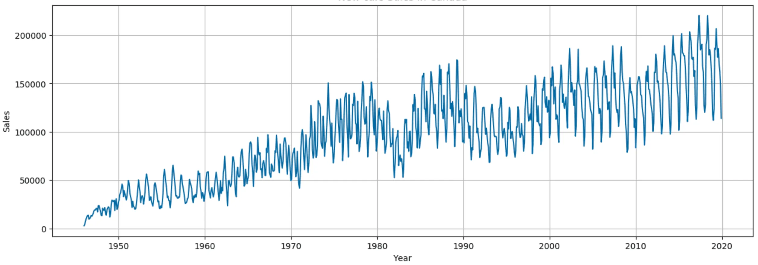
The trend component represents the long-term direction or movement in the time series. It indicates whether the data is generally increasing, decreasing, or staying constant over time.

Characteristics

• Reflects the underlying tendency of the series over a longer period.
• Trends can be linear or non-linear.
• Trends are not affected by short-term fluctuations or irregularities.

Example

In a company’s sales data, a steady increase in sales over several years indicates a positive trend.

2. Seasonal

The seasonal component represents regular, repeating patterns in the time series that occur within a fixed period, such as daily, monthly, or yearly.

Characteristics

• Seasonality occurs at regular intervals and has a fixed period.
• Often driven by external factors such as weather, holidays, or cultural events.
• Seasonal effects are predictable and recur at the same time each year, month, week, or day.

Example

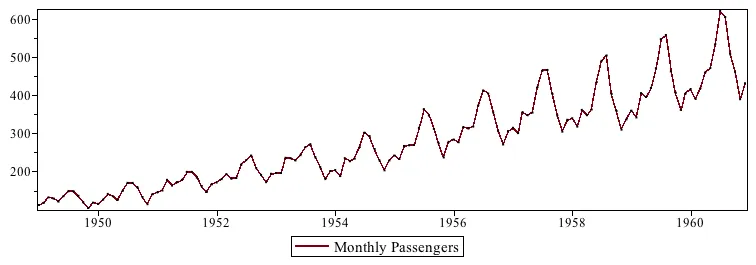
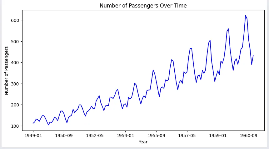
The example here shows the monthly passengers with respect to each month from 1949 to 1960, where we can see the seasonal distribution of the passengers in the chart.

3. Cyclic

The cyclic component refers to fluctuations in the time series that occur over longer periods, usually influenced by economic or business cycles.

Characteristics

• Cycles are usually irregular in period and amplitude.
• They can last for more than a year, often several years.
• Unlike seasonality, cyclic patterns are less predictable in their frequency and duration but are influenced by broader economic factors.

Example

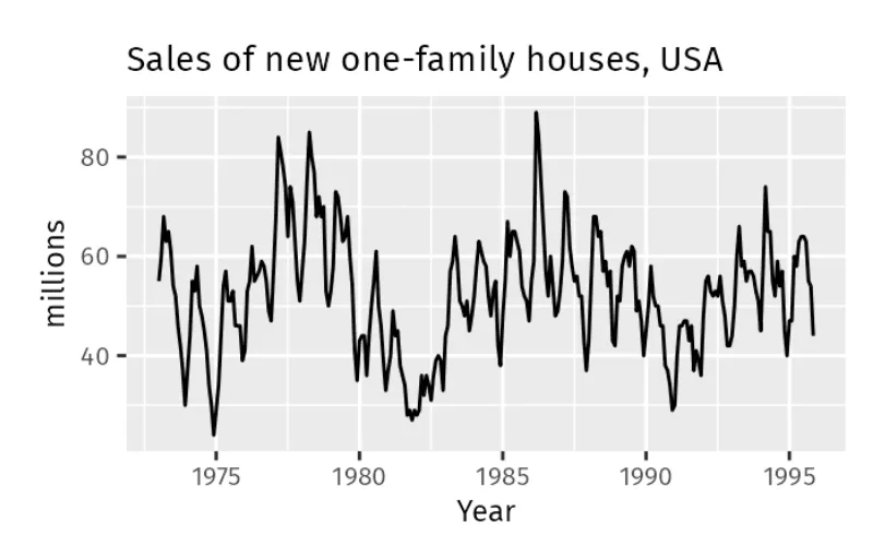
Sales of new family houses fluctuate during certain periods, but these changes are not seasonal, as seen in the graph. These fluctuations could be influenced by periods of economic expansion and recession, which are less predictable than seasonal patterns.

4. Noise

The noise component captures the random variation in the time series that cannot be attributed to trend, cyclic, or seasonal patterns. It represents the unpredictable, irregular fluctuations in the data.

Characteristics

• Noise is the residual part of the time series after removing trend, cyclic, and seasonal components.
• Random and unpredictable.
• Noise does not follow any specific pattern and can be caused by random factors or measurement errors.

Example

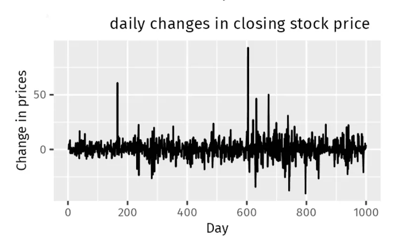
As we can conclude from the graph, there is no specific trend, seasonality, or cyclical pattern in the changes in the stock price of the company. The price fluctuations appear as random ups and downs with no predictable pattern.

Stationarity

Stationarity refers to a characteristic of time series data where the statistical propertie,s such as mean, variance, and autocorrelation, remain constant over time.

• Mean is the average value of observations over a certain time period;
• Variance is the measure of the spread or dispersion of the value around the mean,
• Autocorrelation is the correlation of the series with its previous values.

All the three statistical properties of the time series data should remain constant over time to conclude that the series is stationary. Understanding the series is stationary or not is important, as it informs the type of preprocessing needed to build an effective time series model.When a series is stationary, the recorded values either do not change or stay within the same range over time.

Let’s look at example use cases where the recorded series considered as stationary or non-stationary series.

a. Non-stationary series

A time series data considered non-stationary if the recorded values were affected at different times due to the presence of either trend, seasonality, cyclic or noise in the data.

Example:
Passengers of an Airline will be in increasing trend with seasonal fluctuations every year, as shown in the plot. Hence, this series is considered as non-stationary series.

The ADF test result to assess the presence of stationarity

ADF Statistic: 0.81
p-value: 0.99
Critical Values: {'1%': -3.48, '5%':-2.88, '10%': -2.57}
Fail to reject the null hypothesis: The series is not stationary.

b. Stationary series

When a series is stationary, the recorded values either do not change or stay within the same range over time.

Example:
After applying differential transformation technique of lag 2 , the non-stationary series is converted to stationary series. If we plot the transformed values in a chart, it will appear as shown below:

ADF Test results to assess the presence of stationarity after data transformation

ADF Statistic: -2.96
p-value: 0.03
Critical Values: {
                 '1%': -3.48,
                 '5%': -2.88,
                 '10%':-2.57
                }
Reject the null hypothesis: The series is stationary.

Time series models are typically built using stationary data. If a series is non-stationary, it should be transformed into a stationary series before training the model to ensure accurate future predictions. Two statistical tests, known as the ADF and KPSS tests, are be performed on the time series data to determine whether stationarity is present in the series.

Tests for Stationarity

Stationarity in a time series means that the statistical properties of the series do not change over time. In other words, if you look at different parts of the series, they should look statistically similar. For a series to be stationary, it should have a constant mean, constant variance, and constant auto correlation.

There are two types of statistical methods that can be performed on the time series data to check for the presence of stationarity. They are ADF test and KPSS test. However, before going to stationarity tests, let’s understand a concept in statistical tests called hypothesis.

Hypothesis: Hypothesis testing is a statistical method used to make inferences or draw conclusions about a dataset using sample data drawn from the entire available data. It helps us decide whether there is enough evidence in our sample to support or reject a particular claim or hypothesis about the whole dataset.

• Null Hypothesis (H₀): This is the assumption that there is no effect or no difference. It represents the status quo.
• Alternative Hypothesis (H₁): This is what we want to test for — it’s the opposite of the null hypothesis and represents a new claim or effect.

Now that we understand what the hypothesis mean, let’s look into the stationarity tests:

1. ADF Test

   The Augmented Dickey-Fuller (ADF) test is a statistical test used to determine whether a time series has unit root or not. Presence of unit root indicates that the values are highly dependent on previous values indicates that series is non-stationary.

   Goal: ADF test is used to check if the series contains unit root.

   Null hypothesis: The time series has unit root, hence it is non-stationary.

   Interpretation: If the ADF test statistic is less than the critical value, then the null hypothesis is rejected concluding that the time series is Stationary.

   Testing process: The ADF test works by testing the null hypothesis to check the presence of a unit root in time series indicates that the series is non-stationary.

2. KPSS Test

   The Kwiatkowski-Phillips-Schmidt-Shin (KPSS) test is another statistical test used to check the stationarity of a time series. It differs from the ADF test in that it tests the null hypothesis that the time series is stationary around a mean or a deterministic trend.

   Goal: KPSS test is used to check if the series is stationary.

   Null hypothesis: The time series is stationary around a constant mean or deterministic trend.

   Interpretation: If the KPSS test statistic is greater than the critical value, the null hypothesis is rejected, indicating the series is non-stationary.

   Testing process: The KPSS test examines whether the time series is stationary by testing for a deterministic trend or mean around which it fluctuates.

How to infer the test results

ADF and KPSS tests generate a few statistical values that helps us to classify the series is stationary or not. These values are:

• Test statistic
• P-Value
• Critical Values at 1%, 5%, and 10% Confidence Intervals

Test Statistic

Test statistic is the calculated value in the tests to determine how likely the value would be if the null hypothesis were true.

Calculate the test statistic based on your sample data.

• For a z-test: test statistic is z = (X̄ - μ) / ( σ/ √n) (Statistic value for Whole data)
• For a t-test: test statistic is t = (X̄ - μ) / (s / √n) (Statistic value for Sample data)

Here, X̄ is the sample mean, μ is the population mean, s is the standard deviation of Sample or σ is standard deviation for whole data, n is the sample size.

In QuickML, the ADF and KPSS test statistics are calculated from their respective tests on the whole input data. Both these test statistic values provide a measure of the evidence against the null hypothesis.

The strength of the evidence is assessed at three levels—strong, moderate, and weak—by comparing the test statistic value to the critical values at the 1%, 5%, and 10% significance levels.

P-Value

What is p-Value? The p-value in both tests indicates the probability of obtaining a test statistic value as extreme as the one observed, assuming the null hypothesis is true. P-value can be obtained from the statistical tables to determine whether to the null hypothesis should be rejected.

How is it derived?

1. Formulating and estimating the ADF / KPSS regression model
2. Calculating the test statistics t𝛄 as mentioned above.
3. Comparing t𝛄 against critical values derived from simulation.
4. Interpolating to obtain an approximate p-value based on how the test statistic compares to critical values under the null hypothesis.

In the ADF test

Null hypothesis: The time series has unit root meaning it is non-stationary.

Interpretation: Assuming the significance interval is set as 5%.

1. Low p-value ( ≤ 0.05): A low p-value indicates that you can reject the null hypothesis of a unit root, suggesting that the series is stationary.
2. High p-value ( > 0.05): A high p-value indicates that you failed to reject the null hypothesis of a unit root, suggesting that the series is non-stationary.

In the KPSS test

Null hypothesis: The time series is stationary around a constant mean or deterministic trend.

Interpretation: Assuming the confidence interval is 5%.

1. Low p-value ( ≤ 0.05): A low p-value suggests you reject the null hypothesis indicates that the series is non-stationary.
2. High p-value ( > 0.05): A high p-value suggests you fail to reject the null hypothesis of stationary.

Critical Values (at 1%, 5%, and 10% levels):

Critical values are predefined thresholds or benchmarks used in stationarity tests like the Augmented Dickey-Fuller (ADF) and the Kwiatkowski-Phillips-Schmidt-Shin (KPSS) tests to determine whether to reject or fail to reject the null hypothesis. These values help assess the statistical significance of the test results.

These values serve as benchmarks for decision-making in both KDF and KPSS tests. For example, at 5% significance interval:

• At Critical value at 1%: It is a very strict criterion. If the test statistic value is more extreme than the 1% critical value, then there is a strong evidence to reject the null hypothesis.
• At Critical value at 5%: If the test statistic is more extreme than the 5% critical value, then there is moderate evidence to reject the null hypothesis.
• At Critical value at 10%: It is a more lenient criterion. If the test statistic is more extreme than the 10% critical value, then there is weaker evidence to reject the null hypothesis.

Example:

ADF Test	KPSS Test
Null Hypothesis: The series has a unit root hence it is non-stationary. Example 1: ADF statistic = -3.5 Critical values: CV at 1%: -3.9 CV at 5%: -3.3 CV at 10%: -3.0 Since -3.5 is more extreme than -3.3 (the 5% critical value), you reject the null hypothesis at the 5% level with only moderate evidence. And, if the p-value is 0.04, this confirms you can reject the null hypothesis at 5% confidence interval, since 0.04 < 0.05. Test concludes the series is stationary.	Null Hypothesis: The series is stationary. Example 1: KPSS statistic = 0.6 Critical values: CV at 1%: 0.73 CV at 5%: 0.46 CV at 10%: 0.34 Since 0.6 is greater than the 5% critical value (0.46), you reject the null hypothesis of stationarity at the 5% level with only moderate evidence. If the p-value is 0.02, it means you can reject the null at the 5% level, since 0.02 < 0.05. Test concludes the series is non-stationary.
Example 2: ADF Statistic: 3.14 p-value: 1.0 Critical values: CV at 1%: -3.46 CV at 5%: -2.87 CV at 10%: -2.57 The p-value is greater than the significance level 0.05 and ADF statistic is far greater than all the critical values, hence there is no sufficient evidence to reject the null hypothesis. This concludes that the series is non-stationary.	Example 2: KPSS Statistic: 1.65 p-value: 0.01 Critical values: CV at 1%: 0.73 CV at 5%: 0.46 CV at 10%: 0.34 Reject the null hypothesis: The series is not stationary. The test statistic (1.65) is greater than the critical value (0.46) at the 5% level, and the p-value (0.01) is less than 0.05, we reject the null hypothesis. This means that we have strong evidence to conclude that the series is non-stationary.

Possible outcomes of the tests

The following are the possible outcomes of applying both tests.

Outcome 1: Both tests conclude that the given series is stationary – The series is stationary.

Outcome 2: Both tests conclude that the given series is non-stationary – The series is non-stationary.

Outcome 3: ADF concludes non-stationary, and KPSS concludes stationary – The series is trend stationary. To make the series strictly stationary, the trend needs to be removed in this case. Then, the de-trended series is checked for stationarity.

Outcome 4: ADF concludes stationary, and KPSS concludes non-stationary – The series is difference stationary. Differencing is to be used to make the series stationary. The differenced series is then checked for stationarity.

How to address the stationarity present in columns

In QuickML, we will be using both Augmented Dickey-Fuller (ADF) test and Kwiatkowski-Phillips-Schmidt-Shin (KPSS) test as explained above to check the stationarity of each feature in the time series dataset.

QuickML platform offers a set of data transformation techniques helps to transform non-stationary columns in dataset. By transforming these columns into stationary ones, QuickML ensures that the generated models using the transformed data are well-suited to capture underlying patterns and trends.

Two data transformation techniques that are used primarily to address the stationarity present in columns are:

Differencing

Differencing is done by computing the differences between consecutive observations. It can help stabilize the mean of a time series by removing changes in the level of a time series and therefore eliminating (or reducing) trend and seasonality.

Order of differencing indicates that the number of times the differencing needs to be performed on the non-stationary series to transform it into stationary series. Max order of differencing to be provided in QuickML is 5. If even after the fifth order of differencing the series is non-stationary, any of the methods in power transformations can be applied to stabilize the variance in the time series.

Power transformation

A power transform will make the probability distribution of a variable more Gaussian. This is often described as removing a skew in the distribution, although more generally, it is described as stabilizing the variance of the distribution. Apart from the log transformation, we can use a generalized version of the transform that finds a parameter (lambda) that best transforms a variable to a Gaussian probability distribution.

In QuickML, there are two types of power transformations available

• Box Cox Transformation
  The Box-Cox transformation aims to find the best power transformation of the data that reduces skewness and stabilises variance. It is effective when data exhibits heteroscedasticity (unequal variance across levels of predictors) and/or skewness.
• Yeo Johnson Transformation
  The Yeo-Johnson transformation is a modification of the Box-Cox transformation that can handle both positive and negative values of the target variable. Like Box-Cox, Yeo-Johnson transforms data to stabilize variance and normalize distributions. It is more flexible, as it can handle negative values. Yeo-Johnson is often preferred when the data includes zeros or negative values, which the original Box-Cox cannot handle.

A parameter in the Yeo-Johnson transformation, often referred to as lambda, is used to control the nature of the transform. DIfferent transformation techniques are selected based on the lambda value.

• lambda = -1. is a reciprocal transform.
• lambda = -0.5 is a reciprocal square root transform.
• lambda = 0.0 is a log transform.
• lambda = 0.5 is a square root transform.
• lambda = 1.0 is no transform.

Model evaluation metrics

Metrics for Forecasting

When evaluating forecasts in time series analysis, several metrics are commonly used to assess the accuracy and performance of the model. Each metric provides different insights into how well the forecasted values align with the actual observed values

1. Mean Absolute Percentage Error (MAPE)

MAPE expresses the average absolute percentage difference between predicted and actual values relative to the actual values. It provides insight into the relative accuracy of the forecasts and is particularly useful when comparing the accuracy of models across different datasets or scales.

Interpretation:

For example MAPE value is 8% indicates that the model is relatively accurate as it’s predictions deviate, on average, by 8% from the actual values. Generally, MAPE values below 10% indicates that model is highly accurate, between 10-20% is good, and values above 20% may indicate the need for model performance improvement.

2.Symmetric Mean Absolute Percentage Error (SMAPE)

SMAPE addresses the issue of asymmetry in MAPE by using the average of the absolute values of the actual and predicted values in the denominator. It’s often preferred when dealing with small or zero values in the dataset, as it avoids division by zero and provides a more balanced measure of accuracy.

Interpretation:

SMAPE offers a balanced perspective on error, particularly useful when actual values are small or zero. By using the average of the actual and predicted values in the denominator, SMAPE mitigates the impact of asymmetry. A lower SMAPE value indicates a smaller percentage difference between the actual and predicted values, signaling better model accuracy. It provides a symmetric measure that avoids the issues of extreme percentage errors present in other metrics like MAPE.

3. Mean Square Error (MSE)

MSE measures the average of the squares of the errors, giving more weight to large errors. It provides a more detailed insight into the spread of errors but can be heavily influenced by outliers due to the squaring operation. MSE is useful for penalising larger errors more significantly.

Interpretation:

MSE highlights the variance of errors, with larger errors receiving more weight due to the squaring function. This metric is particularly sensitive to outliers, making it ideal for cases where we want to penalize large deviations from the actual value. A lower MSE indicates a model with fewer and smaller errors on average, though it can be disproportionately affected by outliers. It is useful for understanding the spread of error but may not be as interpretable in real-world units.

4. Root Mean Square Error (RMSE)

RMSE is the square root of the MSE and is more interpretable in the same units as the original data. Like MSE, RMSE gives a measure of the average magnitude of the error, with higher values indicating larger average errors. It is widely used and provides a good balance between sensitivity to error size and interpretability.

Interpretation:

RMSE provides an average error magnitude, retaining the same units as the original data, which makes it more interpretable than MSE. RMSE is sensitive to large errors and is commonly used to understand typical prediction errors. A lower RMSE value indicates a model with lower error and better predictive accuracy. It is useful for models where interpreting errors in terms of the original data units is helpful, giving a clear sense of the “size” of errors.

5. Mean Square Log Error (MSLE)

MSLE calculates the mean of the squared differences between the natural logarithm of the predicted values plus one and the natural logarithm of the actual values plus one. It penalizes underestimates more heavily than overestimates.

Interpretation:

MSLE focuses on the ratio of predicted to actual values, dampening the impact of large values by applying a log transformation. This metric penalizes under-predictions more than over-predictions, making it suitable for models where underestimates are more detrimental than overestimates. A lower MSLE value implies that the predicted values align closely with the actual values on a logarithmic scale, reducing the penalty for high variance in large values and emphasizing performance on a multiplicative scale.

6. Root Mean Square Log Error (RMSLE)

RMSLE is simply the square root of MSLE. It provides a more interpretable measure in the same units as the target variable.Like MSLE, RMSLE penalizes underestimates more heavily than overestimates due to the squared differences.

Interpretation:

RMSLE is the square root of MSLE, preserving the interpretability in terms of the original units, though on a logarithmic scale. Like MSLE, RMSLE penalizes under-predictions more heavily, providing a measure that prioritizes errors in the lower range. A lower RMSLE value suggests closer alignment between predicted and actual values on a log scale, ideal when large positive discrepancies are tolerable but underestimations need to be minimized.