Anomaly Detection
Introduction
Anomaly detection is the process of identifying data points, events, or patterns that deviate significantly from the expected behavior in a dataset. These unusual observations, also called outliers, can indicate critical situations such as fraud, equipment malfunctions, cybersecurity threats, or unexpected shifts in consumer behavior.
In QuickML, we broadly use unsupervised learning algorithms for anomaly detection, where algorithms learn patterns of normality without relying on predefined labels. Instead of being explicitly told what constitutes an anomaly, the algorithm builds an understanding of normal behavior and highlights data points that do not fall within the usual expected range. This makes anomaly detection especially valuable when anomalies are rare, labels are unavailable, or normal patterns are highly dynamic.
Imagine a dataset of credit card transactions. Most transactions follow a typical pattern in terms of amount, frequency, and location. However, a sudden high-value purchase in a foreign country might be flagged as an anomaly. Detecting this anomaly in real time can prevent fraud, protect customers, and save costs for financial institutions.
Business Impact of Anomaly Detection
Anomaly detection is a business-critical process that enables organizations to protect assets, improve operations, and enhance decision-making. Below are some key reasons why anomaly detection is essential across industries:
-
Fraud detection: In finance and e-commerce, anomalies often correspond to fraudulent activities. For example, an unusually high-value purchase made from a foreign location, when compared to a customer’s usual spending behavior, could be an early sign of credit card fraud. Identifying these patterns in real time prevents financial loss and safeguards customer trust.
-
Predictive maintenance: In manufacturing and industrial settings, machines continuously generate sensor data. Detecting anomalies in vibration, temperature, or pressure readings can indicate early signs of mechanical wear or failure. Predicting and addressing these anomalies before they lead to breakdowns significantly reduces downtime and maintenance costs.
-
Cybersecurity and network protection: Anomaly detection helps identify irregularities in system logs, network traffic, or user activity that may indicate a cyberattack, data breach, or unauthorized access. For instance, a sudden surge in login attempts or data transfer volume can reveal security threats that require immediate attention.
-
Healthcare and life sciences: In healthcare, anomaly detection can monitor patient vitals, lab results, or medical imaging data to flag potential health risks. For example, a sudden drop in oxygen saturation or an irregular heartbeat pattern can alert doctors to intervene before the condition becomes critical.
-
Operational insights and decision support: Organizations can use anomaly detection to uncover hidden insights that improve efficiency and support decision-making. For example, unusual spikes in website traffic may reveal marketing campaign success or unexpected customer interests.
What Causes Data Anomalies?
Data anomalies can emerge from a variety of underlying causes, often depending on the nature of the data and the environment in which it is collected. The main contributing factors include:
-
Human error: Manual data entry mistakes, incorrect labeling, or improper configuration of systems can easily introduce irregularities. For example, a misplaced decimal point or an incorrect date format can significantly distort analysis results. Even simple oversights, such as forgetting to update a record or duplicating entries, can lead to anomalous data points.
-
System failures: Hardware malfunctions, software glitches, or communication breakdowns between systems can corrupt or distort data. For example, a temporary network outage during data transmission might result in incomplete or duplicated entries, while a software bug could generate unexpected values or inconsistencies.
-
Fraudulent or malicious activity: In areas like finance, cybersecurity, or e-commerce, anomalies often signal potential fraud or unauthorized access. Abnormally high-value transactions, unusual login patterns, or sudden shifts in user behavior may indicate deliberate attempts to exploit or manipulate the system.
-
Environmental or external changes: Unexpected shifts in external conditions, such as economic fluctuations, market volatility or seasonal changes can alter normal data patterns. These events introduce new variables that cause temporary or permanent deviations from established trends.
Types of Anomaly Detection
Anomalies can be categorized into several types depending on the nature and context of the data. The following sections explain each type in detail with corresponding visualization and conceptual examples.
- Point anomalies
A point anomaly occurs when a single observation deviates significantly from the rest of the data. These are the most common anomalies and are typically easy to detect.
For example, in a dataset of credit card transactions, a sudden high-value transaction may be flagged as a point anomaly if it does not align with the user’s previous spending behavior.
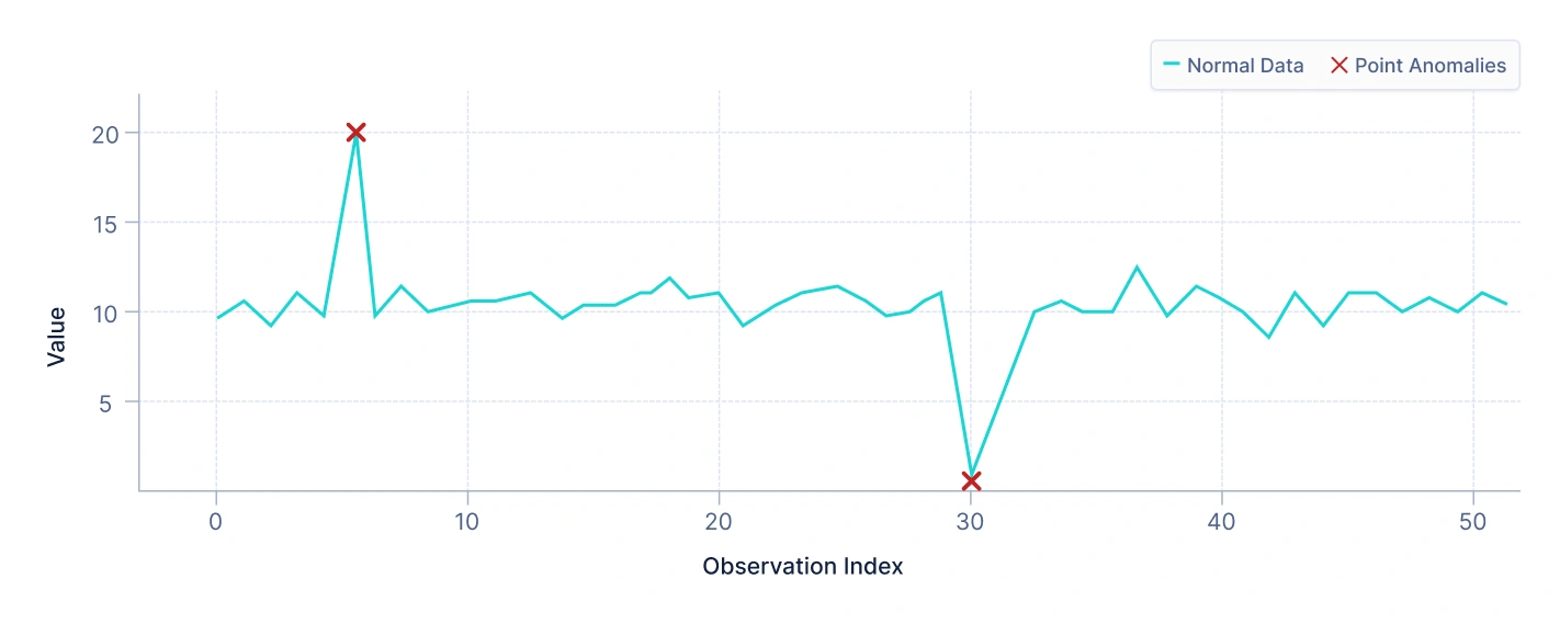
Interpretation: The plot above illustrates how a few data points lie far away from the main data cluster. These isolated data points are clear examples of point anomalies because they differ substantially from the majority of normal data points.
- Contextual anomalies
A contextual anomaly is an observation that is considered anomalous only within a specific context. This type of anomaly is especially common in datasets where the same value may be normal under certain conditions but abnormal under others.
For example, a temperature reading of 10°C may be normal in winter but would be an anomaly in summer. Similarly, an online store may see a high number of purchases during holiday sales, but the same number on an ordinary day could signal suspicious activity.
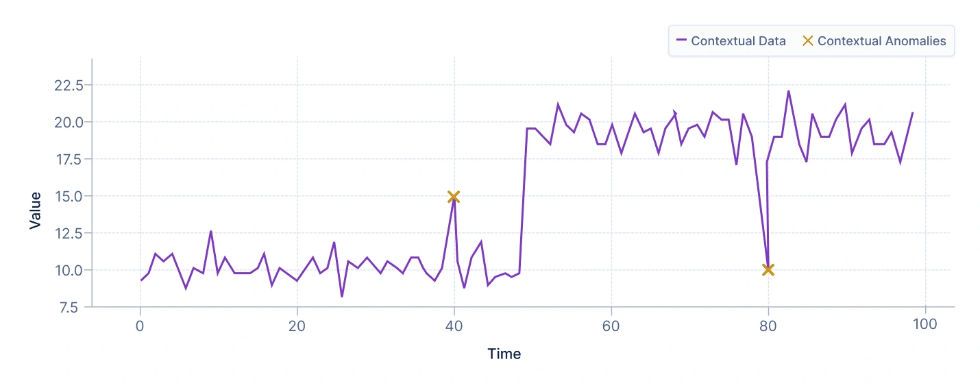
Interpretation: The plot illustrates two distinct contexts, each represented by a separate cluster of data points. These clusters reflect different patterns or environments in which the data behaves normally. The highlighted point lies near one of the clusters, appearing normal when compared to the overall dataset or when evaluated in the context of the other cluster. However, within its own cluster, (when analyzed relative to the specific characteristics and distribution of points in its local context), the point stands out as unusual. This situation highlights a contextual anomaly, where an observation is considered anomalous only within a particular context or under specific conditions, even though it may seem normal in a broader or different context.
- Collective anomalies
A collective anomaly arises when a group of related data points together behave unusually, even if individual points appear normal.
For example, in stock market data, a consistent drop in the stock price of a company over several consecutive days could represent a collective anomaly, especially if this pattern deviates from normal fluctuations.
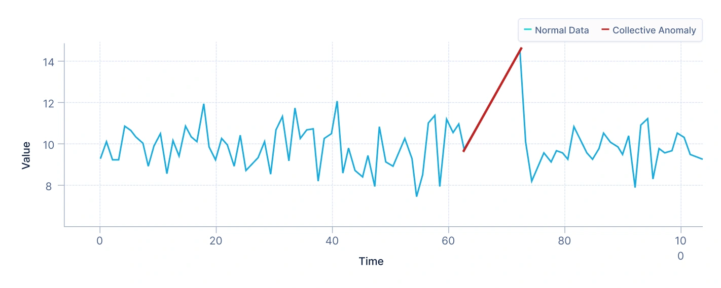
Interpretation: The plot above depicts a small group of points that form a distinct cluster separate from the majority of data. While each individual point within this group may appear normal when evaluated on its own, their collective behavior reveals a pattern that deviates significantly from the overall distribution. This indicates the presence of a collective anomaly, where the anomaly arises not from individual data points, but from their relationship to one another and to the rest of the dataset.
Categories of Anomaly Detection
In QuickML, there are two broad categories of anomaly detection: Time series anomaly detection and Non-time series anomaly detection. Each of these approaches focuses on identifying outliers in different types of datasets, depending on whether time plays a role in the data’s structure.
Here’s a comparison table showing the difference between Time-Series and Non-Time-Series Anomaly Detection:
| Feature | Time-Series Anomaly Detection | Non-Time-Series Anomaly Detection |
|---|---|---|
| Data Structure | Data points are indexed by time and follow a sequential order. | Data points are not indexed by time and are treated as independent observations. |
| Temporal Dependency | Requires algorithms that account for temporal dependencies, trends, and seasonality. | Assumes data points are independent with no temporal relationship. |
| Detection Method | Anomalies are detected by comparing actual values against historical patterns or forecasts. | Anomalies are detected by evaluating similarity or distance between data points in feature space. |
| Influencing Factors | Influenced by seasonality, trends, and long-term dependencies in time. | Influenced by feature relationships and data distribution across multiple variables. |
| Common Algorithms | ARIMA, LSTM Autoencoders, Prophet, Isolation Forest (time-based). | Isolation Forest, One-Class SVM, DBSCAN, LOF. |
| Example Use Cases | Monitoring stock prices, machine sensor readings, network performance over time. | Detecting fraudulent transactions, defective products, or abnormal customer behavior. |
| Key Focus | Focuses on pattern deviations over time. | Focuses on feature-based outliers without considering time. |
Now that we understand the key differences between time-series and non-time-series anomaly detection, let’s explore each of these approaches in depth to gain a clearer and more comprehensive understanding.
Time Series Anomaly Detection
Time series anomaly detection deals with data that is collected and organized in a sequential manner, where each data point is associated with a specific timestamp. This type of data reflects how values change over time, such as stock prices, server performance metrics, sensor readings, or website traffic. Because time is an inherent part of the dataset, detecting anomalies involves analyzing temporal patterns like trends, seasonality, and sudden deviations.
In time series anomaly detection, the goal is to identify moments when the behavior of a system changes unexpectedly compared to its historical pattern. These anomalies can appear as sudden spikes, sharp drops, or irregular fluctuations that break from the usual rhythm of the data.
Time series anomaly detection methods often use forecasting models that learn from past trends to predict expected future values. If the actual observation deviates significantly from the predicted value, the system flags it as an anomaly
Building Intuition Behind Time-Series Anomaly Detection
In time-series datasets, observations are ordered in time, meaning each data point may depend on previous values. Detecting anomalies involves understanding temporal patterns, trends, and seasonality, in addition to feature relationships. The goal is to identify points or periods that deviate from expected temporal behavior.
-
Temporal pattern perspective: Each observation is part of a sequence, and normal points follow predictable patterns over time, including trends, seasonal cycles, and recurring fluctuations. Anomalies break these patterns and stand out as unusual points or sequences that deviate from expected behavior.
-
Trend and seasonality consideration: Sudden spikes, drops, or shifts from established trends often indicate anomalies. It is essential to account for seasonal changes, because deviations may only be anomalous if they violate expected seasonal patterns. For example, a high sales value might be normal during a holiday season but anomalous during a typical off-season period. Properly modeling trends and seasonality allows the system to distinguish between expected variations and true anomalies.
-
Contextual dependencies: Time-based context is critical because the same value may be normal at one point in time but anomalous at another, depending on the surrounding sequence. Additionally, relationships across multiple time-dependent variables can reveal anomalies that might not be apparent when analyzing a single series in isolation. Considering these multivariate temporal dependencies improves detection accuracy by capturing patterns that emerge only when multiple factors are observed together.
-
Density and distribution over time: Anomalies often occur in regions of low probability within the expected temporal distribution. Points that lie far from the predicted range or historical baseline can be flagged as unusual, and probabilistic approaches such as Gaussian processes or historical distribution modeling can quantify these deviations. By understanding the expected density of observations over time, the model can assign anomaly scores that reflect how unlikely each point is relative to normal temporal behavior.
Key Success Criteria for Time-Series Anomaly Detection
Time-series anomaly detection focuses on sequences of data points over time. Success relies on capturing temporal patterns, trends, and seasonality while providing interpretable and actionable insights. Key criteria for success include:
-
Temporal data understanding: Accurately model trends, seasonality, and short- and long-term dependencies. Quality data preparation: Handle missing timestamps, irregular intervals, and inconsistent sampling rates.
-
Effective feature engineering: Include lag features, rolling statistics (mean, variance), differences, or Fourier transforms to capture temporal behavior.
-
Representative historical patterns: Ensure training data reflects normal temporal variations, including rare seasonal patterns, to reduce false positives.
-
Robust model selection: Choose algorithms capable of capturing temporal dependencies, trends, and seasonality. For example, ARIMA, AutoRegressor, Auto ARIMA, or SARIMA.
Business Applications of Time-Series Anomaly Detection
Time-series anomaly detection has wide-ranging applications across industries, helping organizations identify unusual patterns, prevent failures, and make data-driven decisions by monitoring how values evolve over time.
-
Finance and banking
Time-series anomaly detection in finance and banking is used to monitor sequences of transactions for unusual patterns that may indicate fraud or other irregular activities. Sudden spikes in transfers, abnormal trading behaviors, or atypical account activities can be flagged in real time, allowing banks and financial institutions to investigate suspicious behavior promptly. By analyzing the temporal patterns of transactions, models can distinguish between legitimate seasonal or cyclical activity and genuine anomalies that require attention.
-
IoT and industrial operations
In IoT and industrial operations, time-series anomaly detection plays a critical role in monitoring equipment and production processes. Sensor readings collected over time can reveal early signs of machine failure, deviations in performance, or inefficiencies in production lines. By identifying these anomalies early, organizations can schedule predictive maintenance before breakdowns occur, reduce downtime, and maintain optimal operational efficiency. Detecting irregular temporal patterns also helps prevent costly disruptions and ensures the longevity of equipment.
-
Retail and E-commerce
Time-series anomaly detection is also valuable in retail and e-commerce for monitoring sales, returns, and website activity over time. Sudden drops or spikes in these metrics may point to operational issues, shifts in customer behavior, or fraudulent activity. By analyzing temporal patterns, businesses can distinguish between normal seasonal fluctuations and true anomalies, enabling faster response to unexpected events, improving customer experience, and optimizing operational decisions.
Univariate vs Multivariate Forecasting in Time Series
In time-series anomaly detection, the data being analyzed can either be univariate or multivariate, depending on the number of variables tracked over time. In QuickML, data is categorized this way to ensure that models are applied appropriately: univariate forecasting is simpler and computationally efficient for single-variable trends, while multivariate forecasting is necessary when anomalies arise from interactions between multiple features, which could be missed in a univariate approach. This distinction helps you to choose the right modeling strategy and feature representation for accurate anomaly detection, whether the focus is on a single metric or on complex patterns across several interdependent variables.
It is important to understand the difference between univariate and multivariate data, as this choice directly impacts how anomalies are detected and interpreted in time-series analysis.
| Feature | Univariate Data | Multivariate Data |
|---|---|---|
| Definition | Tracks a single variable over time. | Tracks multiple interrelated variables over time and forecasts a single target variable while accounting for its dependencies on other related variables (multivariate forecasting), similar to how traditional predictive models operate. |
| Focus | Monitors trends, seasonality, and fluctuations of one metric. | Monitors patterns and interactions among multiple metrics simultaneously. |
| Anomaly Detection | Flags deviations in the single variable from expected behavior. | Flags anomalies based on irregularities in relationships between variables, capturing patterns that may not appear in isolation. |
| Complexity | Simpler and computationally efficient. | More complex, requires modeling dependencies and interactions between variables. |
| Use Cases | Website traffic, daily sales, electricity consumption, revenue monitoring. | Retail analytics (sales vs marketing spend), stock market analysis (price, volume, volatility), healthcare monitoring (heart rate, blood pressure, oxygen levels). |
| Strengths | Easy to implement and interpret; good for single-metric monitoring. | Detects subtle anomalies that arise from variable interactions; captures complex patterns. |
How Time-Series Anomaly Detection Works
Let’s go over time-series anomaly detection using the ARIMA (AutoRegressive Integrated Moving Average) model, one of the most widely used forecasting-based methods.
-
Understand the time-series data
The process begins with collecting sequential data points, where each value is linked to a specific timestamp, for example, daily website visits, hourly temperature readings, or minute-by-minute stock prices. Because time is an essential factor, patterns such as trends (overall growth or decline) and seasonality (repeated cycles) are important to identify.
-
Train the forecasting model
ARIMA learns from the historical time-series data to understand its underlying patterns. It combines three components:
- AR (AutoRegressive): Uses past values to predict future ones.
- I (Integrated): Makes the data stationary by removing trends.
- MA (Moving Average): Uses past forecast errors to refine predictions.
The model is trained to capture how the data usually behaves over time.
-
Generate forecasted values
After training, ARIMA predicts what the next data points should look like based on historical patterns. For each timestamp, the model produces an expected (forecasted) value and a confidence interval, which represents the normal range of variation.
-
Compare actual vs. predicted values
The actual observed value from the dataset is then compared to the model’s predicted value. If the observed value lies far outside the expected range (for example, much higher or lower than the forecasted confidence band), it is considered an anomalous point.
-
Detect and report anomalies
Once the entire time series is analyzed, the system flags timestamps where significant deviations occur. For example, a sudden spike in network traffic could indicate a cyberattack. The output typically highlights these timestamps and shows the number of detected anomalies for further investigation.
Example: Imagine a company monitoring its website’s hourly traffic. ARIMA predicts that the next hour should have around 1,200 ± 100 visits, but the actual count drops suddenly to 400.Since this value lies far outside the expected range, the system flags it as an anomaly, prompting the company to investigate potential causes like a server crash or connectivity issue.
Steps to Build a Time Series Anomaly Detection Pipeline
In QuickML, time-series anomaly detection is implemented through the Smart Builder, which is designed specifically for datasets where observations are made over time. The Smart Builder structures this process into four main stages: Source → Preprocessing → Algorithm → Destination.
Stage 1: Source
The pipeline begins with ingesting the timeseries dataset, such as stock prices, machine sensor readings, or daily sales. Since these datasets are sequential, selecting the correct time-based input ensures the system can detect anomalies relative to historical patterns.
Stage 2: Preprocessing
Smart Builder automatically prepares raw time-based data for anomaly detection.
Frequency: For timeseries datasets, data is resampled to a consistent frequency (e.g., daily, weekly). This standardization ensures anomalies are detected across uniform intervals rather than distorted by irregular timestamps.
Imputation: Missing values in the dataset are handled through imputation. Without this step, gaps may be misinterpreted as anomalies or distort the model’s ability to recognize true patterns.
Transformation: Transformation ensures the dataset is adjusted so that anomalies stand out more clearly rather than being hidden by trends or scale effects. In Smart Builder, this step can be configured directly, and users have two main options: Differencing or Power Transformation.
-
Differencing: Differencing works by calculating the difference between consecutive observations in a time series. This process helps stabilize the mean by removing shifts in the series’ level, effectively reducing or eliminating trends and seasonality. The order of differencing specifies how many times this operation is applied to transform a non-stationary series into a stationary one. In QuickML, you can specify a maximum order of differencing up to 5. If the series remains non-stationary even after the fifth order of differencing, you can apply one of the available power transformation methods to further stabilize the variance and make the series suitable for anomaly detection.
-
Power Transformation: Stabilizes variance and normalizes skewed data distributions. This is especially useful when raw data values are spread across very different scales, making anomalies in smaller values harder to detect. Available options for power transformation in Quickml are:
- Log Transformation: Applies a logarithmic scale to compress large values and spread smaller ones. This helps reveal anomalies that might otherwise be overshadowed by extreme outliers.
- Square Root Transformation: Useful when dealing with moderate skewness; it reduces the impact of high values while retaining the relative differences across smaller values.
- Box-Cox Transformation: A flexible option that automatically determines the best power parameter (λ) to stabilize variance and normalize the dataset. Particularly effective when values are strictly positive and the distribution is heavily skewed.
- Yeo-Johnson Transformation: Similar to Box-Cox but also works with zero or negative values, making it more versatile for datasets that aren’t strictly positive.
Stage 3: Algorithm
Once preprocessed, Smart Builder applies algorithms designed for timeseries anomaly detection, such as Isolation Forest or One-Class SVM. These models learn normal temporal behavior and flag deviations as potential anomalies, whether they appear as sudden spikes, drops, or irregular sequences.
Stage 4: Destination
Finally, Smart Builder outputs anomalies along with supporting metrics and visualizations. These results allow users to validate flagged anomalies, interpret the context, and take timely action. The system ensures anomalies are presented in an accessible format for faster decision-making.
Non-Time Series Anomaly Detection
Non-time series anomaly detection deals with data that does not have an inherent temporal order, meaning the individual data points are independent of time or sequence. Each observation is treated as a standalone instance rather than part of a continuous timeline. Examples include credit card transactions, medical records, network packets, product reviews, or manufacturing measurements.
In non-time series anomaly detection, the goal is to identify data points that behave differently from the majority of the dataset. Since there is no time component, detecting anomalies in non-sequential data focuses on spatial, relational, or statistical patterns rather than temporal ones. Methods analyze the distribution and structure of the data, measuring how far each point deviates from the normal population.
Building Intuition Behind Non-Time-Series Anomaly Detection
In non-time-series datasets, observations are static and independent of time. Detecting anomalies involves understanding relationships between multiple features. The goal is to define the boundary that separates normal behavior from abnormal behavior.
-
Feature space perspective: Each observation can be visualized as a point in a high-dimensional space. Normal points cluster together, while anomalies lie far from these clusters.
-
Density-based thinking: Anomalies often occur in low-density regions where few data points exist. Algorithms use this intuition to assign anomaly scores.
-
Multivariate dependencies: Relationships between multiple features must be considered. A point might appear normal along individual dimensions but be anomalous when combined with other features.
-
Context awareness: In categorical or grouped data, normality can vary between groups. Understanding this contextual variation is essential for accurate detection.
Key Success Criteria for Non-Time-Series Anomaly Detection
Non-time-series anomaly detection focuses on static or independent data points rather than sequences over time. Success depends on accurately identifying abnormal patterns within these static datasets, understanding relationships among features, and providing interpretable and actionable insights. Key criteria for success include:
-
Quality data preparation: Ensure data is clean, consistent, and representative of normal behavior.
-
Effective feature engineering: Choose features that capture meaningful variations in behavior. Combining numerical and categorical attributes provides a richer representation of normality.
-
Representative normal samples: The training data should cover the full range of legitimate patterns to prevent misclassification of valid variations as anomalies.
-
Robust model selection: The chosen algorithm must handle noise, outliers, and different data distributions.
Business Applications of Non-Time Series Anomaly Detection
Non-time series anomaly detection is applied across many industries to identify unusual data points or behaviors that deviate from normal patterns. Because this type of data is not dependent on time, it helps organizations detect rare or suspicious events and strengthen decision-making across a wide range of operations.
-
Healthcare
In healthcare, non-time series anomaly detection is used to find unusual patient records or diagnostic results that may indicate errors, rare diseases, or potential fraud in insurance claims. For example, an unusually high number of procedures for a single patient or medical test results that differ greatly from normal ranges can be flagged for further review. Detecting these irregularities helps improve patient safety, reduce billing fraud, and maintain data accuracy in medical systems.
-
Human Resources and Recruitment
In HR and recruitment, anomaly detection can help identify unusual employee data, such as unexpected salary levels, inconsistent performance metrics, or irregular application patterns. Detecting these outliers helps organizations maintain fairness, detect data errors, and prevent possible policy violations. It also assists in spotting exceptional talent or early signs of workforce issues.
-
Cybersecurity
In cybersecurity, anomaly detection helps identify suspicious network activities or system access patterns that differ from typical user behavior. For example, a login attempt from an unusual location, unauthorized data access, or abnormal file transfers can indicate potential cyberattacks or insider threats. By analyzing the relationships and characteristics of network data, security systems can detect and respond to threats quickly, even without relying on time-based sequences.
How Non-Time Series Anomaly Detection Works
Now, let’s understand non-time series anomaly detection using the Isolation Forest algorithm, a popular method that works well for high-dimensional, tabular data.
-
Understand the dataset
In non-time series data, each record is treated as an independent observation with multiple features (for example, customer age, income, and spending score). There’s no timestamp or sequential order, the goal is simply to find data points that look very different from most others.
-
Build random trees
Isolation Forest creates many random decision trees by repeatedly splitting the dataset into smaller sections. Each split randomly selects a feature and a split value. The idea is that normal data points need more splits to be isolated, while anomalies, being rare and different, get isolated quickly with fewer splits.
-
Measure isolation depth
For every data point, the algorithm calculates the average number of splits (path length) needed to isolate it across all trees.
- If a point is isolated quickly, it is likely an anomaly.
- If it takes many splits, it is considered normal.
-
Compute anomaly scores
An anomaly score is then calculated for each record based on its average path length. Values closer to 1 indicate stronger anomalies, while values near 0 suggest normal behavior.
-
Detect and report anomalies
Finally, the model classifies records with high anomaly scores as outliers and reports the number of anomalies detected in the dataset. These points can then be examined to understand why they differ from the norm, for example, fraudulent transactions or data-entry errors.
Example: Imagine a bank analyzing customer transactions. Most customers spend amounts between $50 and $500, but a few transactions suddenly appear at $10,000+. Isolation Forest isolates these high-value transactions with very few splits, flags them as anomalies, and reports how many such suspicious cases exist, helping the bank focus on potential fraud.
Steps to Build a Non-Time Series Anomaly Detection Pipeline
For non-timeseries data, such as customer transactions, employee records, or survey responses, anomaly detection pipelines are built using Classic Builder. Here, the process skips frequency alignment and temporal transformations, since the data is not sequential. Instead, Classic Builder directly prepares tabular data, applies algorithms, and outputs anomalies that highlight unusual or suspicious records.
By separating Smart Builder for timeseries data and Classic Builder for non-timeseries data, QuickML ensures that each anomaly detection pipeline is tailored to the unique structure of the dataset, improving both accuracy and interpretability.
Stage 1: Data ingestion
The process begins with loading the dataset into QuickML, which serves as the foundation for the anomaly detection workflow. This step involves importing data from various sources such as CSV files, relational databases, APIs, or cloud storage systems. Since non–time series data does not depend on temporal order, each record is treated as an independent observation. Ensuring accurate and complete data ingestion is critical for reliable anomaly detection results.
Stage 2: Data preprocessing
Once the data is imported, it undergoes a preprocessing phase to ensure accuracy, consistency, and readiness for analysis. This step includes handling missing values through imputation or removal and encoding categorical variables using label or one-hot encoding. Effective preprocessing ensures that anomalies reflect true irregularities rather than data quality issues, improving the performance and interoperability of the detection model.
Stage 3: Algorithm selection
After preprocessing, QuickML allows users to select an appropriate anomaly detection algorithm based on the characteristics of the dataset and the nature of expected anomalies. Common approaches include Isolation Forest, One-Class SVM, and Local Outlier Factor (LOF). Each algorithm uses different principles to distinguish normal data from anomalies. Choosing the right method is crucial for accurately capturing the unique patterns and relationships within the dataset.
Stage 4: Model training and detection
In this step, the selected algorithm is trained on the processed data to learn the normal behavior or structure of the dataset. During training, the model identifies typical patterns, boundaries, or distributions and then evaluates each instance to detect those that deviate significantly from the learned norms.
Stage 5: Anomaly reporting
After the model identifies anomalies, QuickML summarizes the results by displaying the number of anomalies detected in the dataset. This output provides a clear overview of how many data points deviate from normal patterns based on the trained model.
Evaluation Metrics in Anomaly Detection
The evaluation metrics below help assess how well the anomaly detection model is identifying deviations from normal behavior and how accurate its underlying predictions are. These metrics quantify prediction error, model reliability, and ultimately the trust you can place in flagged anomalies.
Mean Absolute Percentage Error (MAPE)
What it tells you: MAPE measures how far, on average, the model’s predicted values deviate from the actual observed values in percentage terms. It expresses the size of prediction errors relative to the magnitude of actual data, which makes it intuitive and easy to interpret across different datasets or scales. This metric is particularly useful when you need to understand how accurate your model’s predictions are in terms of percentage deviation rather than absolute difference.
Intuition:
- A lower MAPE indicates that the model’s predictions are closer to the true values.
- A very high MAPE usually signals poor model accuracy — or that actual values are very small, which inflates percentage errors.
Example Inference: If MAPE is 15%, it means predictions deviate from actual values by 15% on average.
Symmetric Mean Absolute Percentage Error (SMAPE)
What it tells you: SMAPE improves on MAPE by treating over-predictions and under-predictions equally. This makes it a fairer and more balanced measure, especially when your dataset contains small or zero values that can distort traditional percentage errors. SMAPE expresses how large prediction errors are compared to the average of the predicted and actual values, ensuring the metric remains stable even when actual values are close to zero.
Intuition:
- SMAPE ranges between 0% (perfect prediction) and 200% (completely inaccurate).
- It is preferred over MAPE when your dataset contains very small or zero values to avoid disproportionately large errors.
Example Inference: A SMAPE of 18.68% indicates that, on average, predictions deviate by 18.68% from actuals in a symmetric fashion, which is a reasonably acceptable level of error for many real-world anomaly detection tasks.
Mean Squared Error (MSE)
What it tells you: MSE calculates the average of squared differences between the predicted and actual values. By squaring the errors, it emphasizes large deviations, meaning big mistakes have a much stronger impact on the score. This makes MSE valuable for understanding how significantly prediction errors vary across the dataset and for identifying models that may be making large, costly errors.
Intuition:
- An MSE of 0 means perfect predictions.
- Higher MSE values indicate a higher level of prediction error.
- Because errors are squared, large deviations contribute disproportionately, making MSE sensitive to outliers.
Example Inference: In the provided output, MSE is 0, meaning the model’s predictions match the observed values exactly, which is an ideal case.
Root Mean Squared Error (RMSE)
What it tells you: RMSE is the square root of MSE and provides an error measure in the same unit as the original data, making it more interpretable. It represents the standard deviation of prediction errors, or how spread out the residuals are around the true values. RMSE is especially helpful when comparing models or assessing prediction consistency.
Intuition:
- RMSE is easier to interpret than MSE because it is expressed in the same unit as the predicted variable.
- Lower RMSE means better prediction accuracy.
Example Inference: An RMSE of 0.0041 indicates that, on average, the prediction error is very small and close to the true values.
Mean Squared Log Error (MSLE)
What it tells you: MSLE measures the squared difference between the logarithms of predicted and actual values. Instead of focusing on absolute differences, it emphasizes relative errors, making it ideal for data that spans multiple scales or involves exponential growth (e.g., population, sales, or web traffic). MSLE rewards predictions that are proportionally close to actual values and penalizes underestimation more strongly than overestimation, which is useful when missing a spike is more serious than over-predicting one.
Intuition:
- MSLE penalizes underestimation more than overestimation.
- Best used when your data spans multiple orders of magnitude (e.g., exponential growth patterns).
Example Inference: An MSLE of 0 indicates perfect alignment between predicted and actual values in log scale, meaning no significant under- or over-prediction.
Root Mean Squared Log Error (RMSLE)
What it tells you: RMSLE is the square root of MSLE, making it easier to interpret while retaining its focus on relative prediction accuracy. It helps evaluate how much the model’s predictions differ from actual values in percentage-like terms without being overly influenced by large outliers. RMSLE is particularly useful for problems where relative growth or proportional differences are more important than exact numerical accuracy.
Intuition:
- RMSLE is less sensitive to large absolute errors but emphasizes relative accuracy.
- Particularly useful when percentage differences matter more than raw differences.
Example Inference: An RMSLE of 0.0041 indicates that, on a log scale, the prediction errors are extremely low, confirming high-quality forecasting.
Number of Anomalies
What it tells you: This metric represents the count of data points flagged as anomalies by the model after processing the dataset. It provides a direct measure of how frequently the system detects deviations from normal behavior.
Intuition:
- A very high number of anomalies might indicate that the model is too sensitive (many false positives).
- A very low number might mean the model is too strict and missing meaningful anomalies.
Example Inference: If the model detects 42 anomalies, you can review them to ensure they correspond to meaningful events, like sudden demand spikes or sensor failures, and not random noise.
How to use these metrics together
No single metric tells the full story of model performance. Use them collectively to get a holistic view; prediction error metrics (MAPE, SMAPE, MSE, RMSE, MSLE, RMSLE) indicate how accurately the model forecasts normal behavior, while the number of anomalies shows how often the model flags deviations.
Example: Suppose your model has an RMSE of 0.0041, a MAPE of 15%, and detects 42 anomalies in a dataset. The low RMSE and moderate MAPE indicate that predictions are very close to actual values, and the number of anomalies is reasonable, suggesting the model is accurate and appropriately sensitive. If instead the model flagged 300 anomalies, you might suspect it’s too sensitive and producing many false positives.
Interpreting these metrics together helps balance prediction accuracy with meaningful anomaly detection, giving you confidence in actionable insights.
Visual Evaluation of Anomalies
Visual evaluation is a crucial step in validating the performance of a time-series anomaly detection model. It enables qualitative assessment of the model’s outputs by comparing predicted anomalies against the actual time-series behavior. This visualization enables users to:
- Quickly validate whether detected anomalies align with real changes in the data.
- Identify false alarms or missed anomalies.
- Gain insight into the model’s reliability across different time segments and trends.
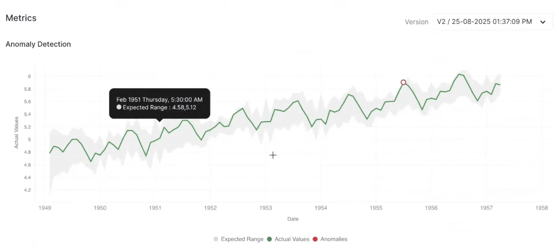
What it tells you: This visualization shows how the model identifies anomalies in a time-series dataset. The chart plots actual data values over time, highlights the expected (normal) range, and marks points that deviate significantly as anomalies.
Intuition:
- Green line: Represents the actual observed values over time.
- Gray shaded area: Indicates the expected or predicted range of normal behavior based on the model.
- Red circles: Highlight points detected as anomalies, where the actual values significantly deviate from the expected range.
- If the red anomaly points align with clear spikes, drops, or deviations outside the gray expected range, it indicates that the model is accurately capturing unusual patterns.
- Few, well-placed anomalies suggest the model is stable and precise.
- Frequent or random anomaly points within normal regions may indicate an overly sensitive threshold or noise in detection.
Example: If anomalies appear at sharp peaks in the series (e.g., sudden increases in values), it suggests genuine outliers or unexpected events. If anomalies appear during normal fluctuations, it may indicate that the model needs threshold adjustment to reduce false positives.
Last Updated 2025-11-11 12:15:26 +0530 IST
Yes
No
Send your feedback to us