Create Time Series Pipeline

Now that the dataset is uploaded, we’ll create a time series pipeline using the uploaded dataset.

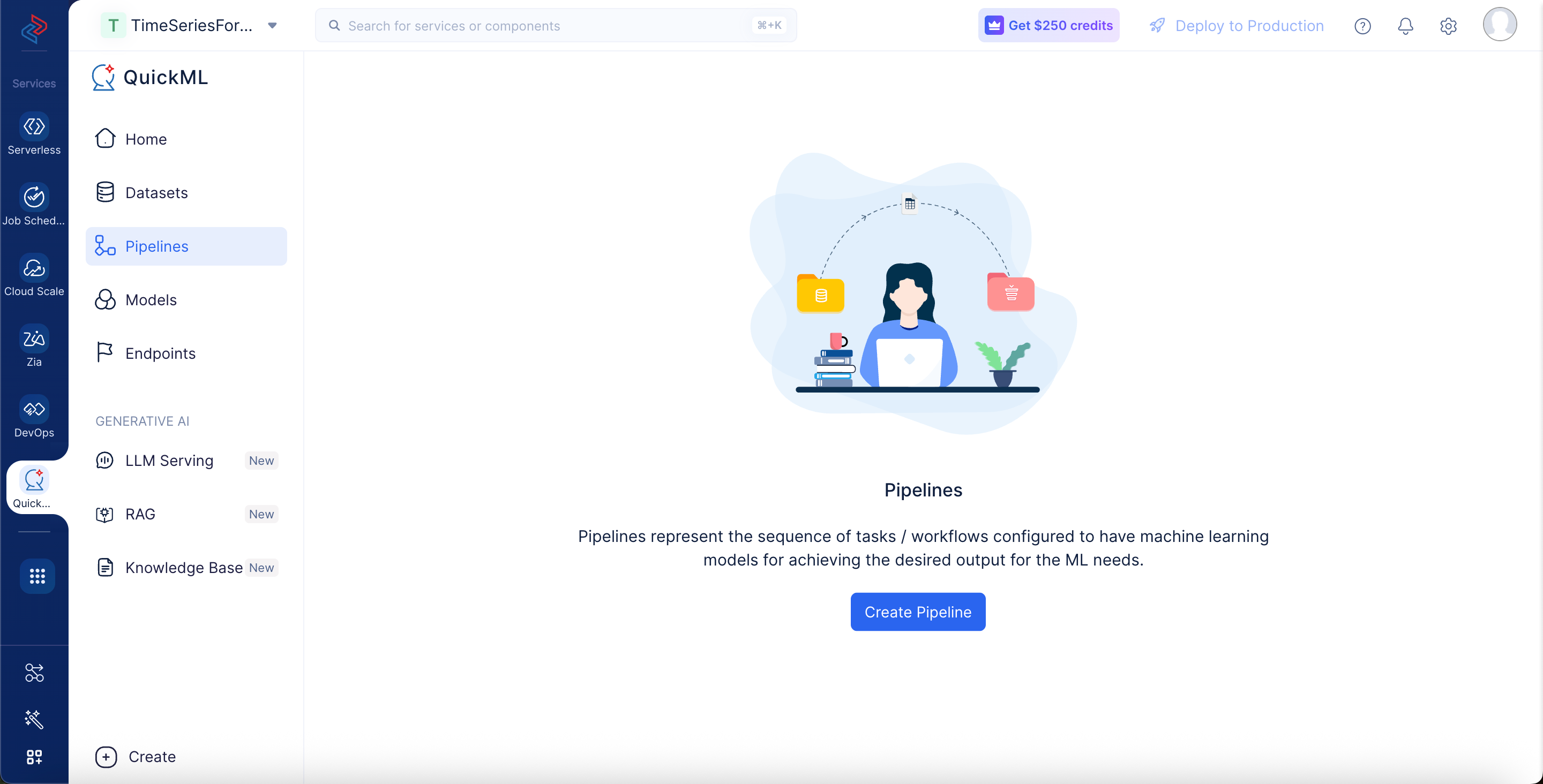
1. Navigate to the Pipeline component in the left menu and click on the Create Pipeline button.

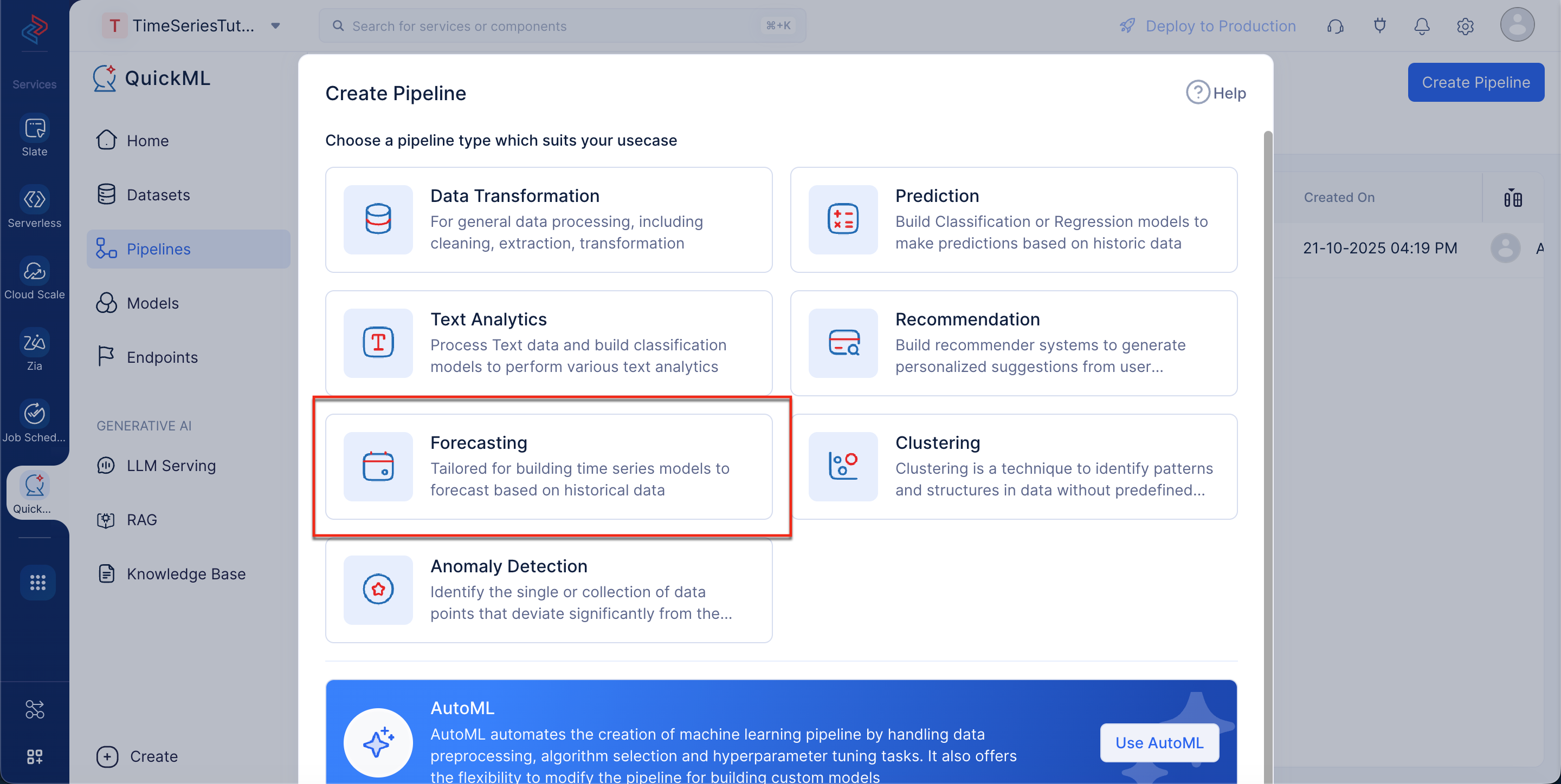
2. In the Create Pipeline window, select the Forecasting pipeline model.

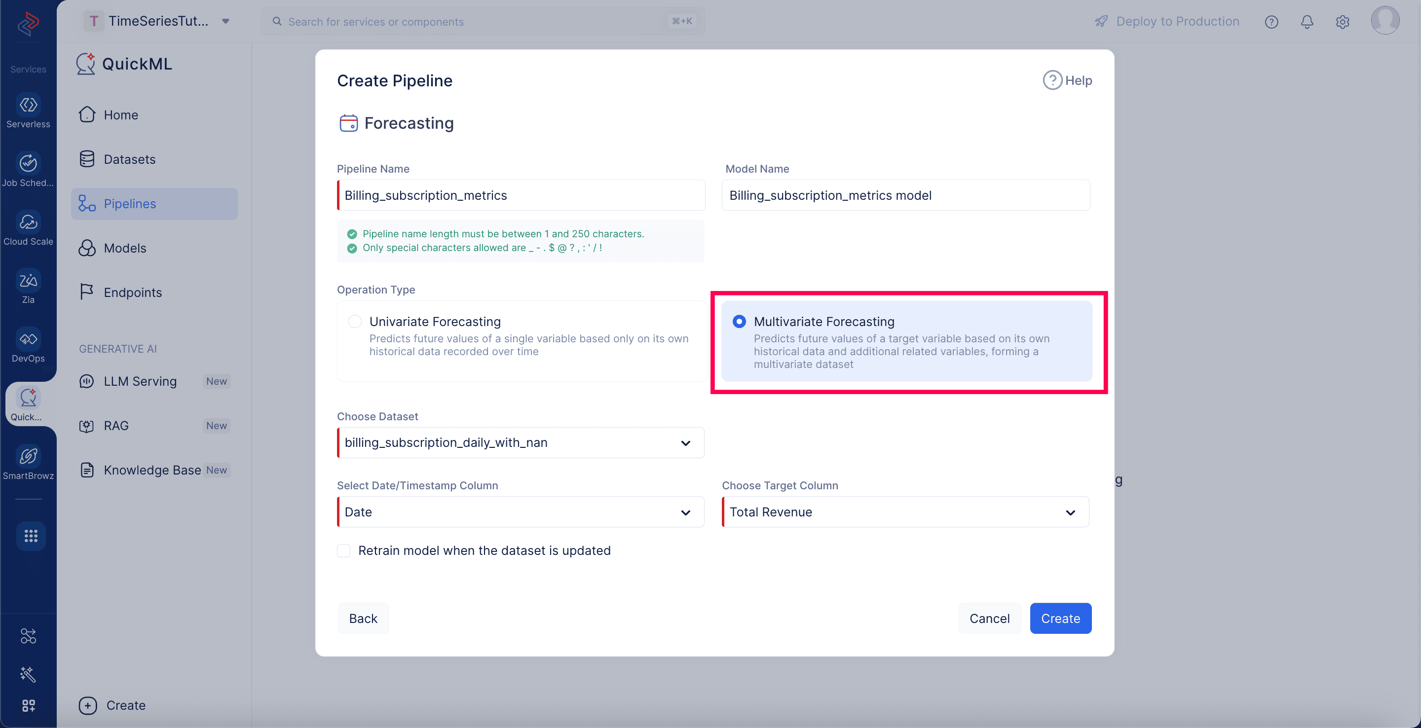
3. Name the pipeline as billing_subscription_metrics, set the operation type to Multivariate Forecasting, and choose the billing_subscription_metrics dataset from the dataset drop-down. After selecting the dataset, specify the date as the Date/Timestamp column and total revenue as the Target column. Click Create to create the pipeline.

You’ll land on the Time Series smart mode pipeline builder as seen in the below image. This is a pre-built pipeline template with required operations to build a forecasting pipeline seamlessly in a short time.

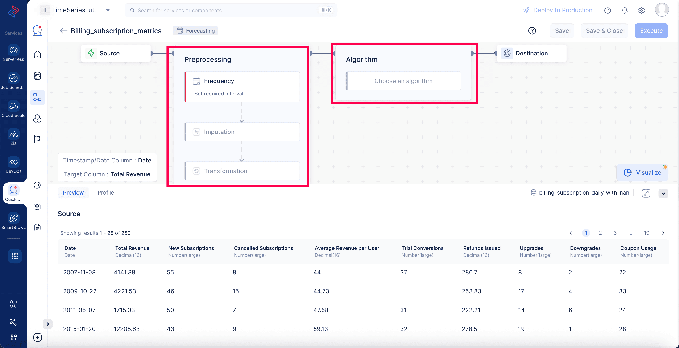
The smart mode pipeline builder contains two main stages: Preprocessing and Algorithm, in the pipeline template as shown above.

Also, if you navigate to the Profile tab in the builder beside the sample preview, there’s an option to show the profile for sample data and whole data.

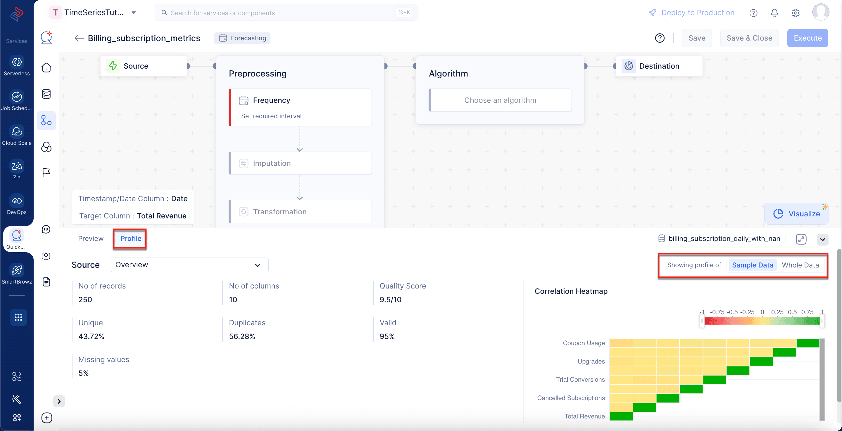
The profile for the sample data is generated by default after configuring each operation in the pre-processing and algorithm stages, but in case you need a profile of the whole dataset during the pipeline building process, select Whole Data and click Generate.

The first step in building any ML model is data preprocessing. In the Smart Builder, we have predefined preprocessing operations required for time series data.

Below are the list of operations to be configured in the preprocessing stage for our multivariate forecasting model:

• Frequency: Daily (1-day interval)

• Imputation: Fill in missing values in the Target column

• Transformation: Square Root Transform—Yeo Johnson

Let’s go through each stage and understand why it’s necessary to configure the model.

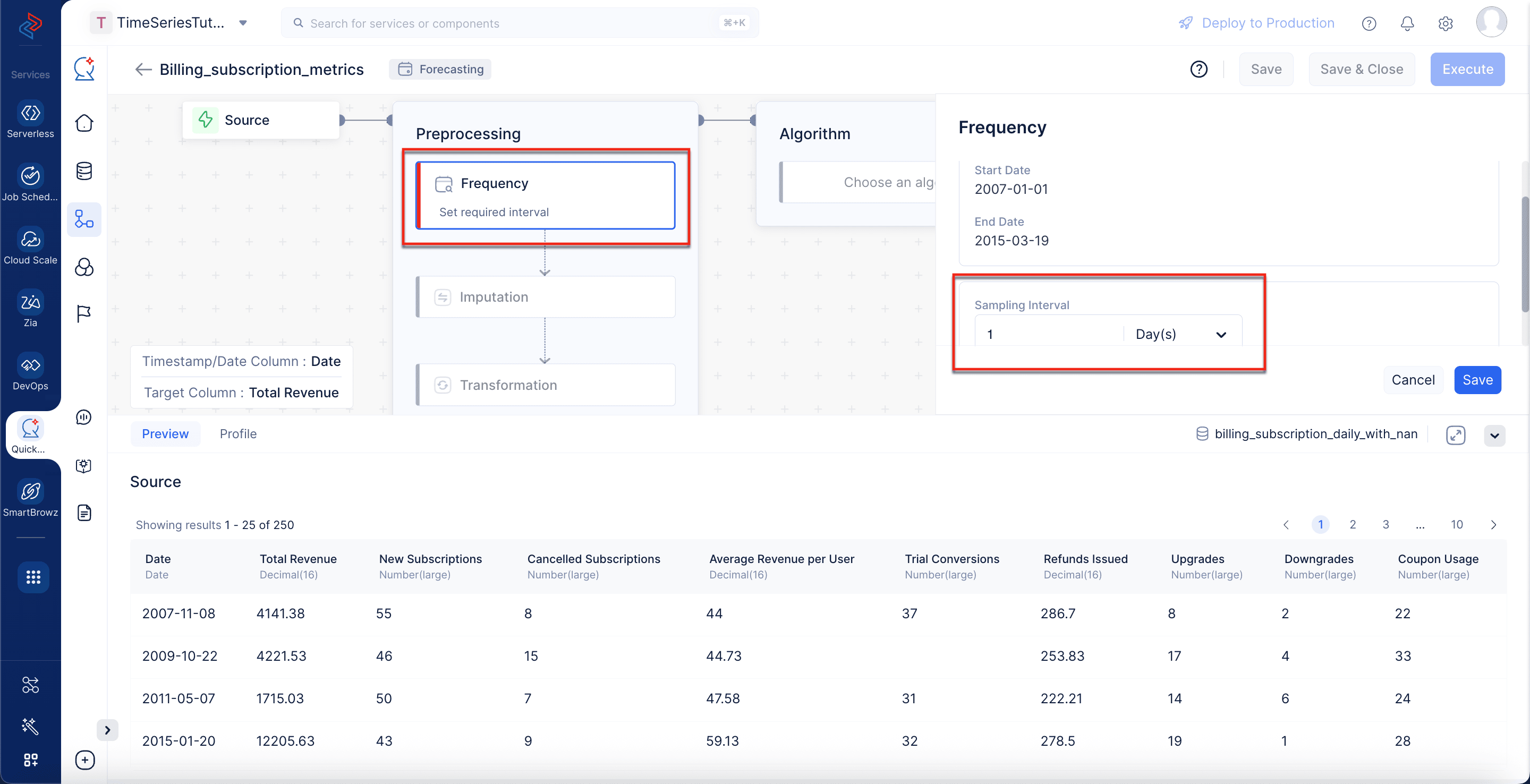
Time series data must follow a consistent time interval. Frequency alignment ensures that all records are uniformly spaced.

Here, select the interval as 1 Day because the dataset contains daily billing subscription metrics. This ensures that the model can learn from a continuous daily sequence without irregular gaps. Once the frequency is set, click Save and Run the frequency operation.

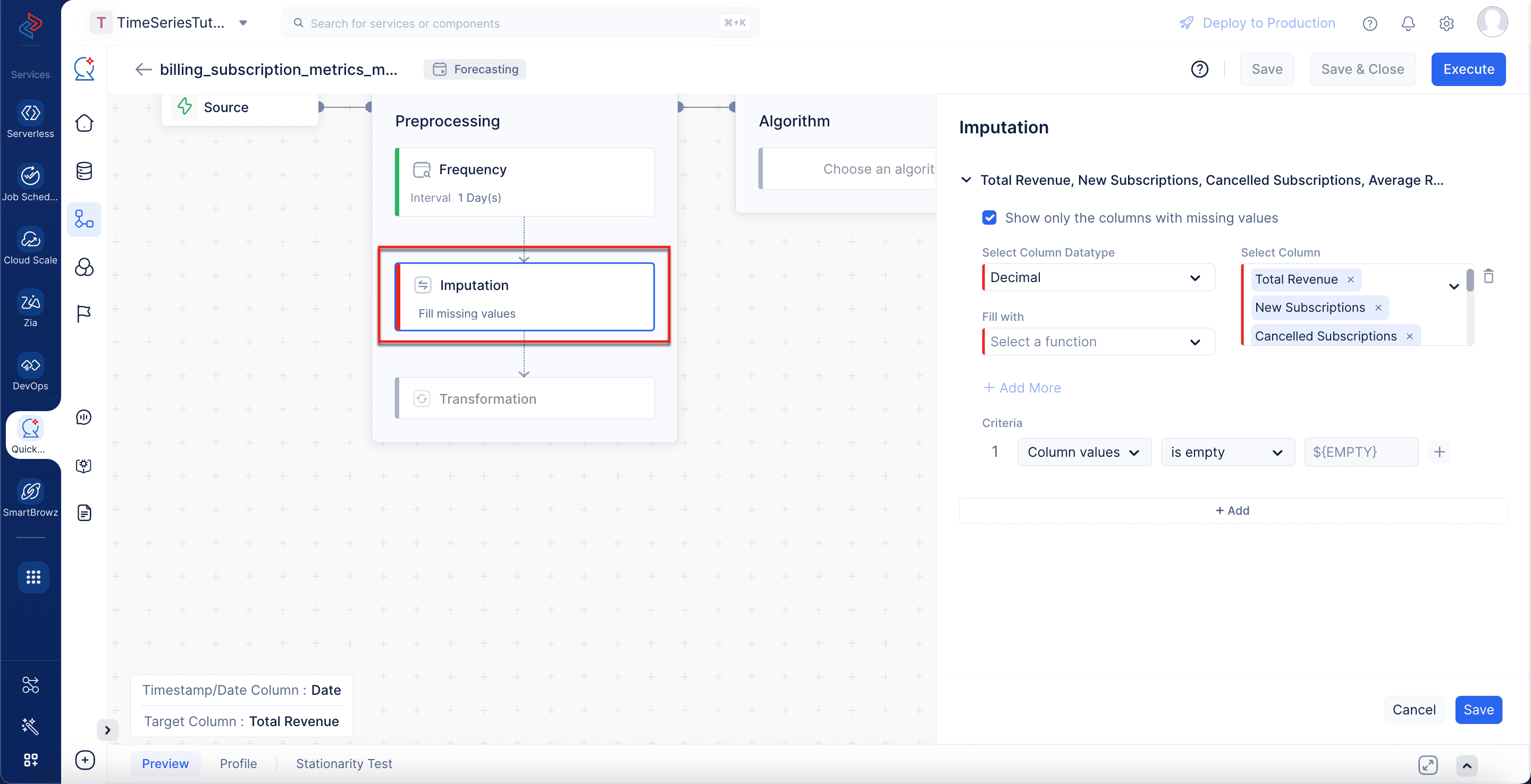
Real-world time series data often contains missing values. Imputation is used to fill in these gaps so the sequence remains consistent.

Here, the target column, Total Revenue—along with all other columns with missing values—are selected with datatype Decimal, and missing values are filled in using the mean of the available values. This approach fills in missing values in a way that maintains the overall continuity and trend of the time series, without distorting the data from sudden spikes or drops. Once the imputation is handled, click Save and Run the imputation operation.

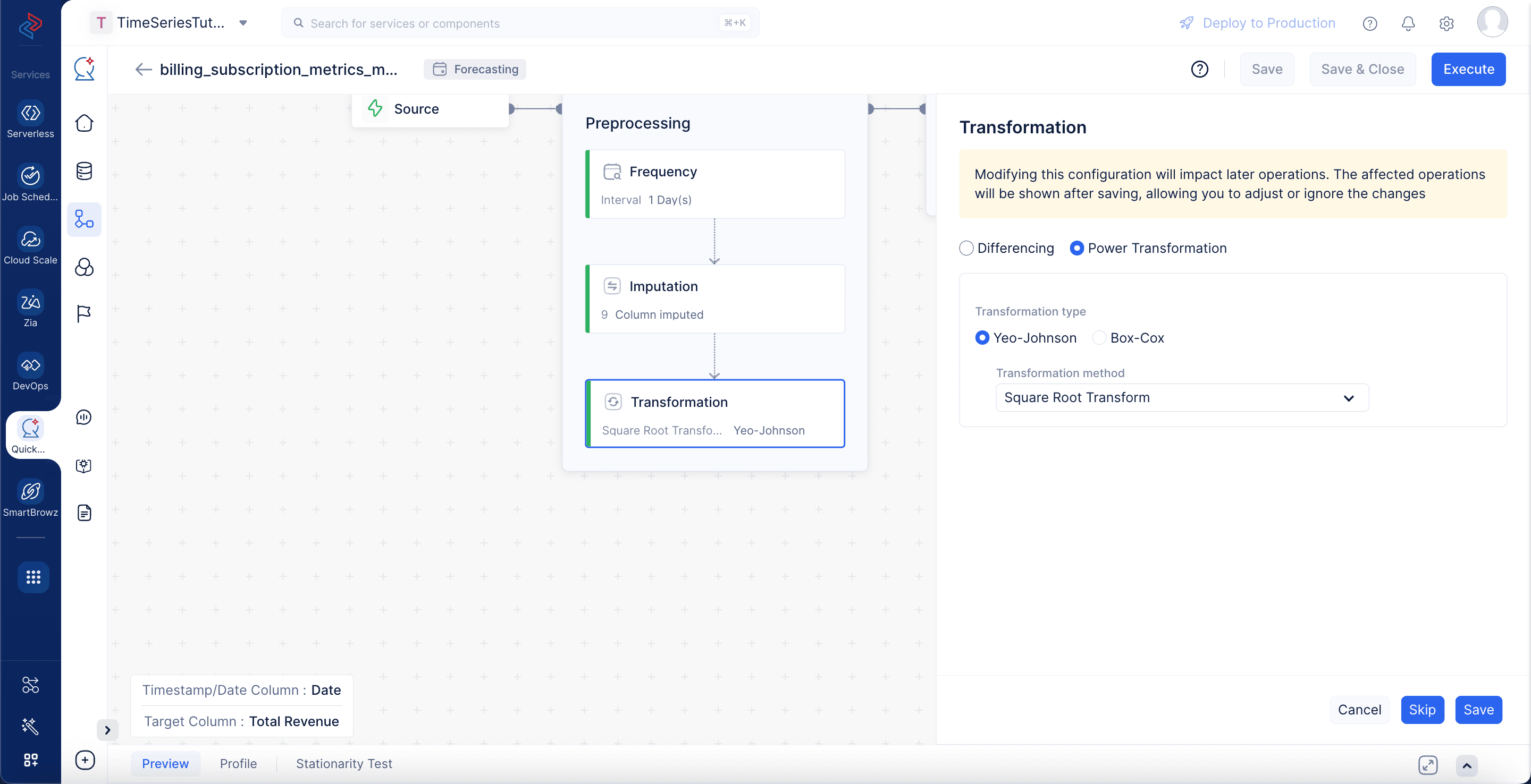
Transformation refers to applying statistical data transformation techniques to the data (such as log transformation or differencing) in order to stabilize variance or stationarity. In this pipeline, a Square Root–Yeo Johnson power transformation is applied to normalize the data distribution and reduce skewness. This helps the model handle non-linear relationships more effectively and improves overall forecasting accuracy. Once the transformation is configured, click Save and Run the transformation operation.

Upon executing the transformation operation, you can find the Stationarity Test tab appearing next to the Preview and Profile tabs. Click the Stationarity Test tab to view the results of the stationarity analysis performed on the transformed dataset.

This tab helps you evaluate whether each time series feature in your dataset is stationary or non-stationary using two statistical tests—KPSS (Kwiatkowski-Phillips-Schmidt-Shin) and ADF (Augmented Dickey–Fuller). These tests are essential to verify that the data has a stable mean and variance over time indicates that the time-series is stationary, which is a necessity for forecasting models.

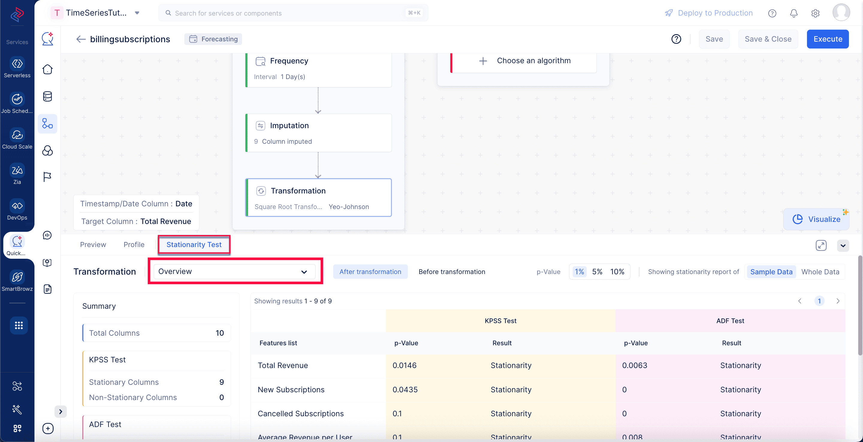
You can gain certain stationarity insights using the below options.

• Transformation stage overview: Located at the top left, this dropdown (set to Overview by default) lets you choose which transformed feature or dataset view you want to analyze for stationarity. You can select Overview to see the results for all columns together, or pick a specific feature such as Total Revenue, New Subscriptions, or Cancelled Subscriptions, to view detailed stationarity results for that individual column. Depending on the transformations applied (for example, Square Root, Yeo-Johnson, Log, or Differencing), the dropdown allows you to explore how each transformation impacts the stationarity of the selected variable.

• After/Before transformation toggle: Right next to the dropdown, you’ll see two options: Before transformation (shows results on the raw data) and After transformation (shows results on the data after applying your transformation steps). In the screen below, After transformation is selected, showing that all features have become stationary after processing.

• p-Value Significance Selector: Located toward the top center of the panel, this option lets you choose the significance level used to determine whether a feature is stationary. You can switch between 1%, 5%, or 10% thresholds depending on how strict you want the stationarity test to be. Note: Changing this value updates the Result column (Stationary/Non-Stationary) in both KPSS and ADF test results accordingly.

  • 1%: Very strict, only very small p-values indicate stationarity.

  • 5%: Standard threshold, commonly used in statistical testing.

  • 10%: More lenient: useful when working with noisy or short time series.

    Learn about the significance of p-Value here

• Sample Data/Whole Data toggle: Located on the upper right side, this toggle allows you to decide whether the stationarity tests should run on a subset of your dataset or on the entire dataset. In the displayed screen, Sample Data is selected, meaning the stationarity report is generated using a sampled portion of the data.

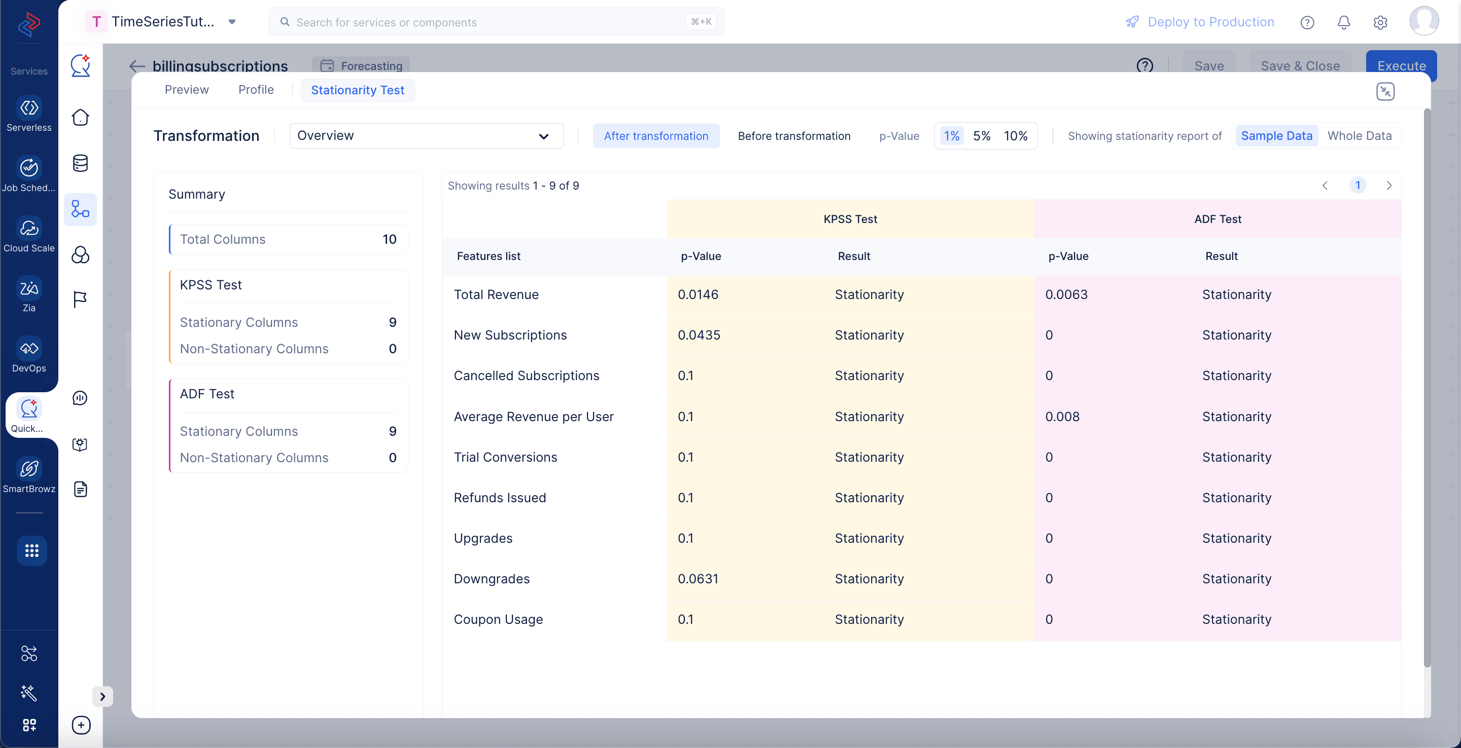
• Summary panel: Shown on the left side of the Stationarity Test tab, this panel provides a quick summary of how many features are stationary or non-stationary based on each statistical test. Total Columns displays the total number of time-series features analyzed. KPSS Test shows the number of columns classified as stationary or non-stationary according to the KPSS test. ADF Test shows the same classification results according to the ADF test. The underlying assumption is that the series should be made stationary according to both tests to help ensure a well-performing model.

• Results table: Located in the main area of the screen, this table lists the detailed test results for each column in the dataset. It contains the following:

• Features list: The names of each time series feature tested (e.g., Total Revenue, New Subscriptions, etc.).

• KPSS p-Value and Result: The p-value and outcome from the KPSS test; higher p-values generally indicate stronger evidence of stationarity.

• ADF p-Value and Result: The p-value and outcome from the ADF test; lower p-values generally indicate stronger evidence of stationarity.

Now that the preprocessing stage configuration is completed, the dataset is ready for training. In the next step, the VAR algorithm will use this processed data to model the target variable and generate the corresponding forecasts.

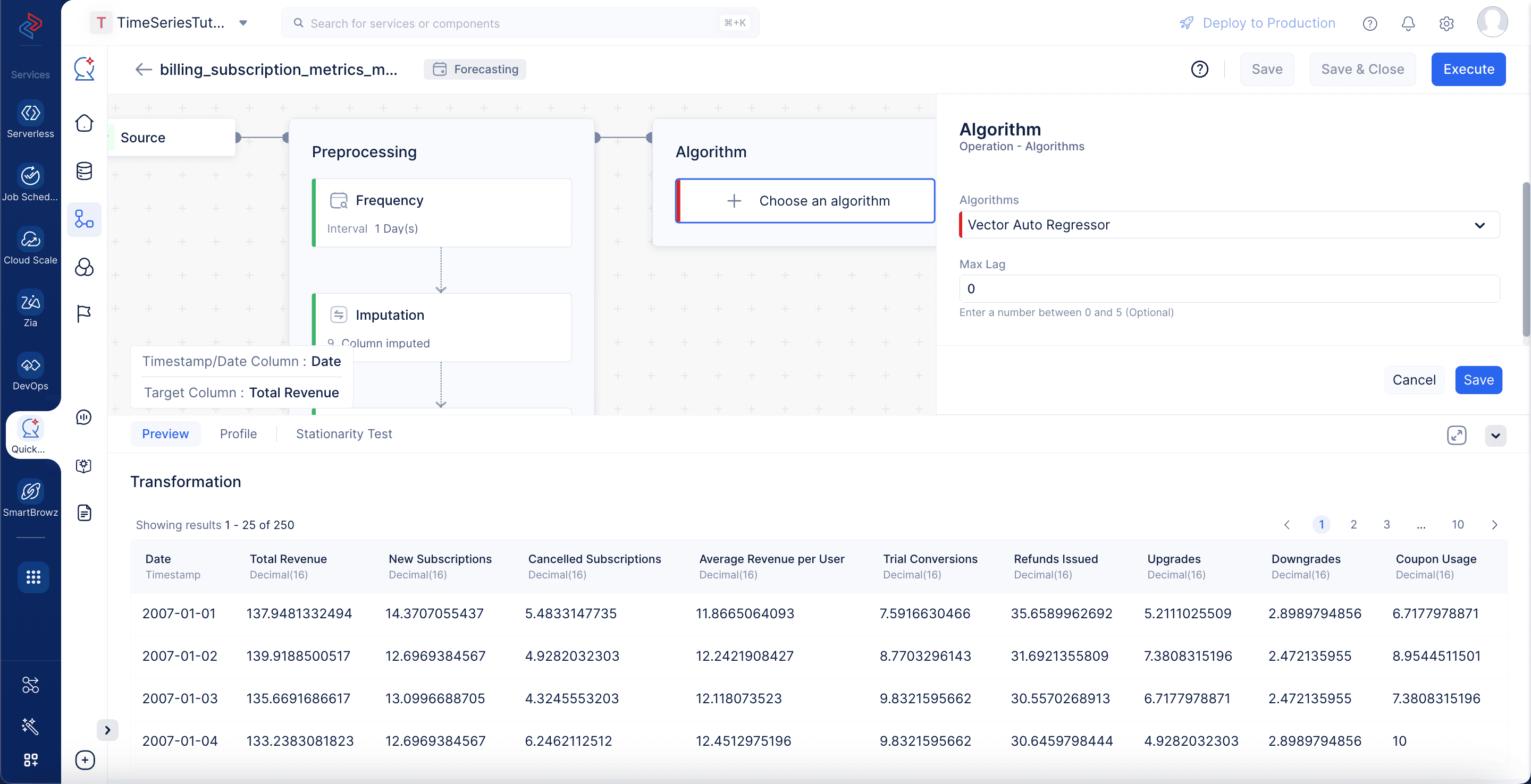
After preprocessing the dataset, the next step is to configure and apply the forecasting algorithm. In this tutorial, we use VAR, a robust multivariate time series algorithm that captures relationships among multiple interdependent variables. VAR simultaneously analyzes several related variables; for example, Total Revenue, New Subscriptions, Cancellations, and Refunds, to understand how changes in one metric influence the others over time.

In our parameter configuration, Max Lag is set to a value between 0 and 5. This parameter determines how many previous time steps (lags) the model will use to predict future values. Selecting an appropriate lag value helps the model capture temporal dependencies effectively while preventing overfitting.

Here, click the Algorithm stage, choose VAR from the drop-down and retain with the given parameter configuration. Then, click Save.

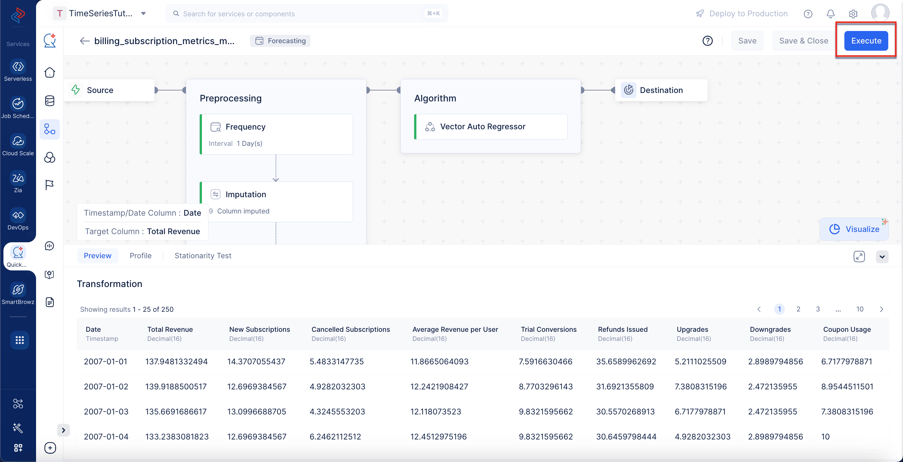
Now, execute the pipeline by clicking the Execute button at the top-right corner of the pipeline builder page.

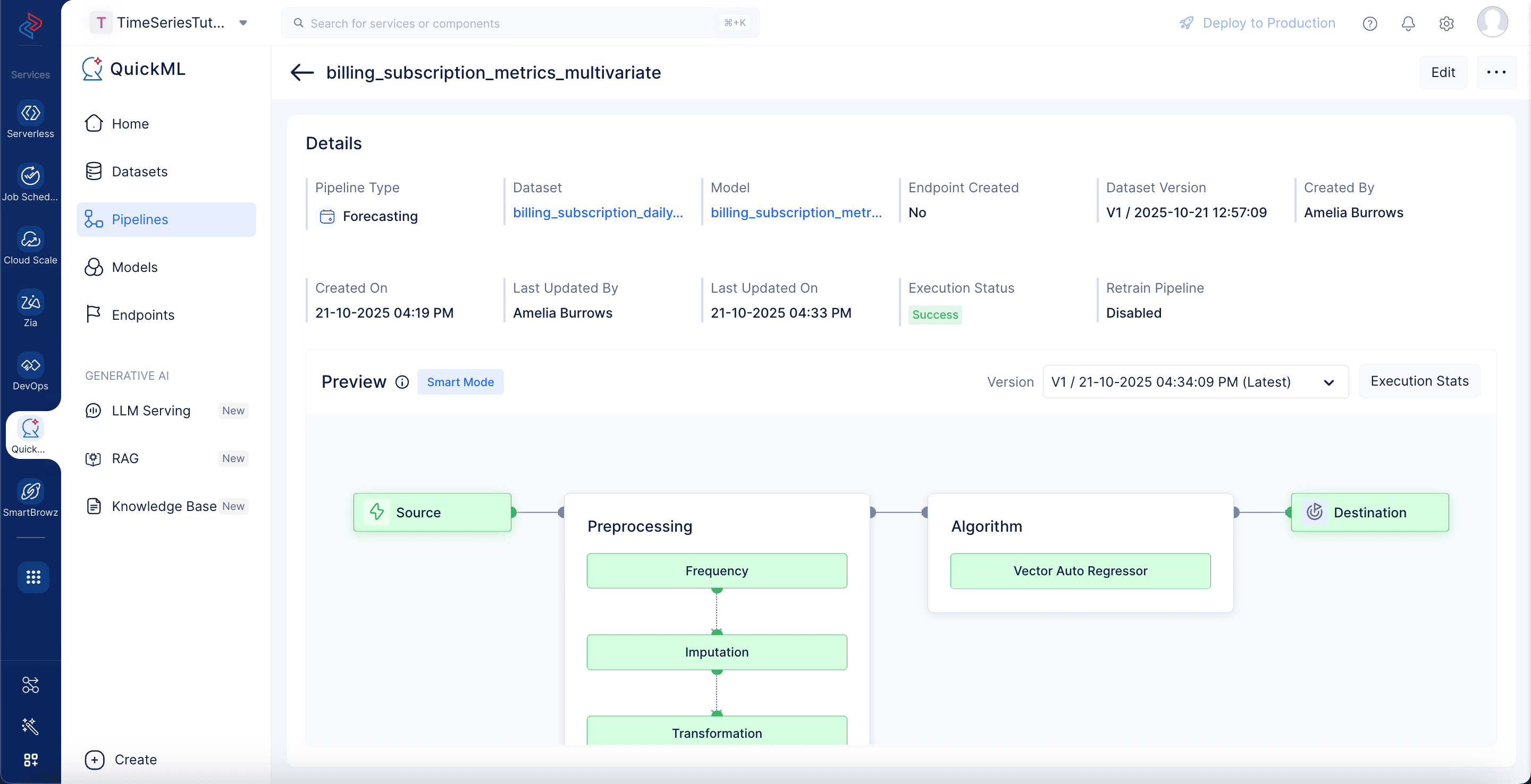
This will redirect you to the pipeline details page shown below, which provides details about the executed pipeline with execution status. You can see that the pipeline execution is successful.

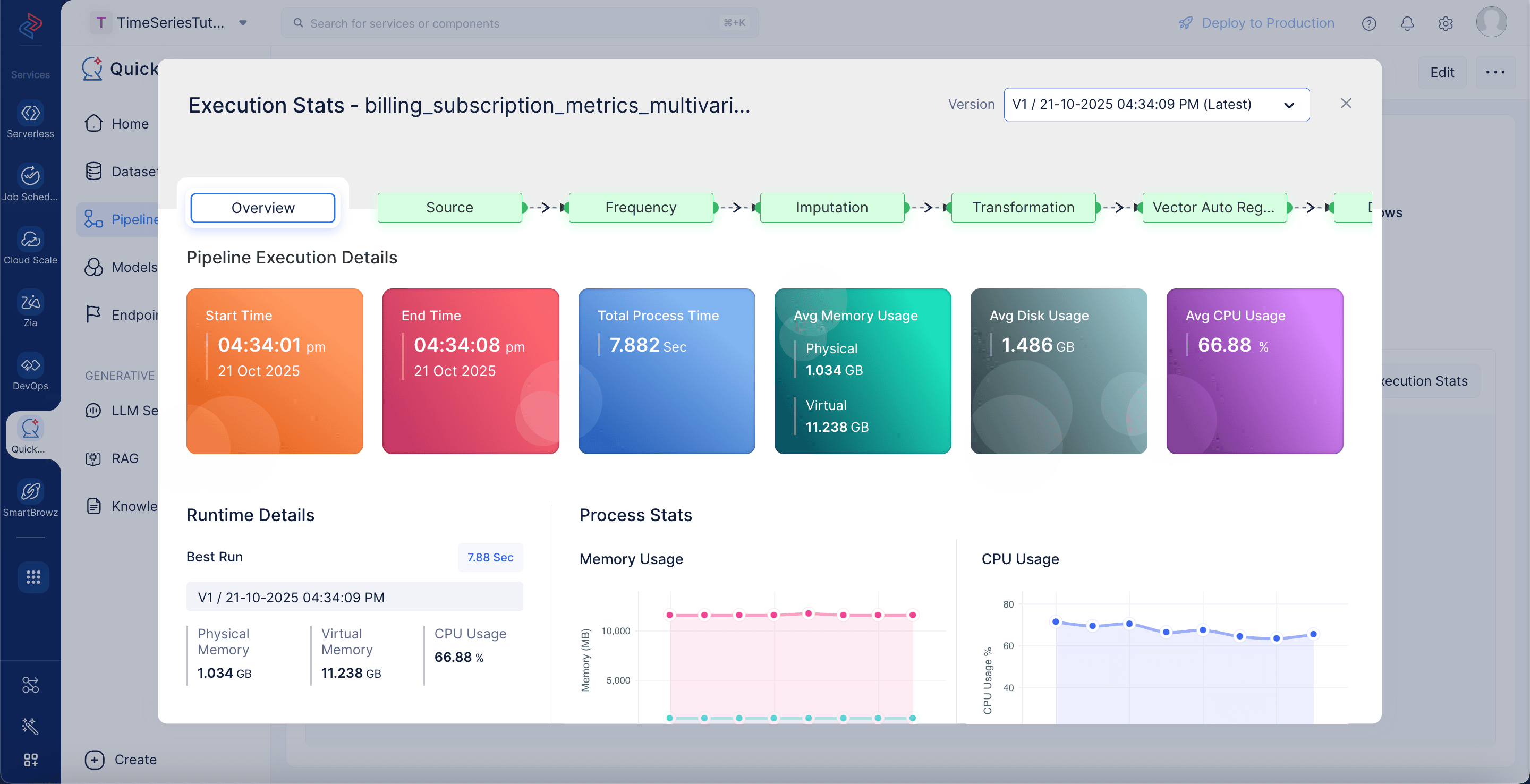
Click Execution Stats to view more details about each stage of the model execution.

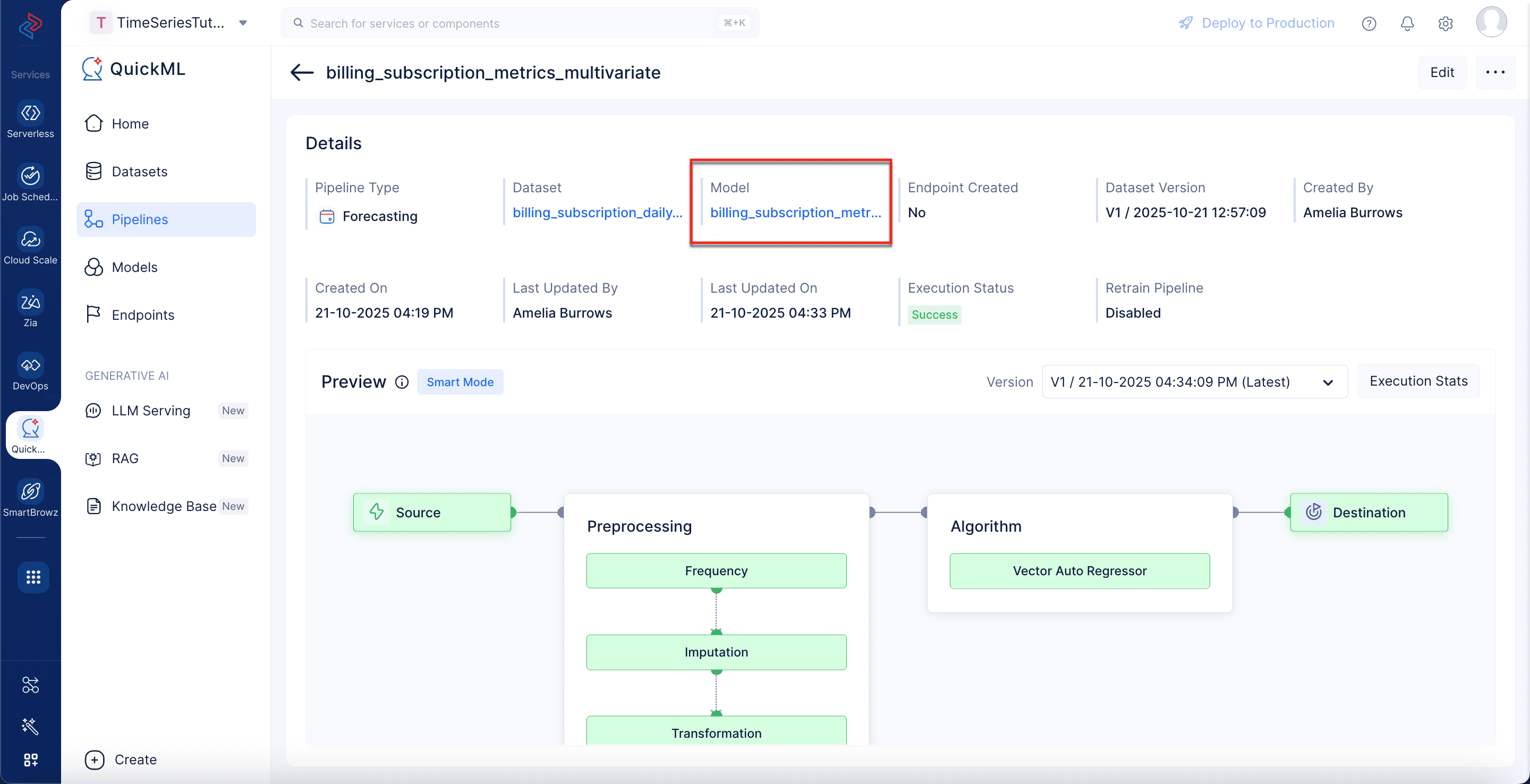
The time series forecasting model is ready to analyze the billing subscription metrics for the OTT platform, and its details can be accessed under the Model field. (Click on the billing_subscription_metrics_model following the successful execution of the pipeline.)

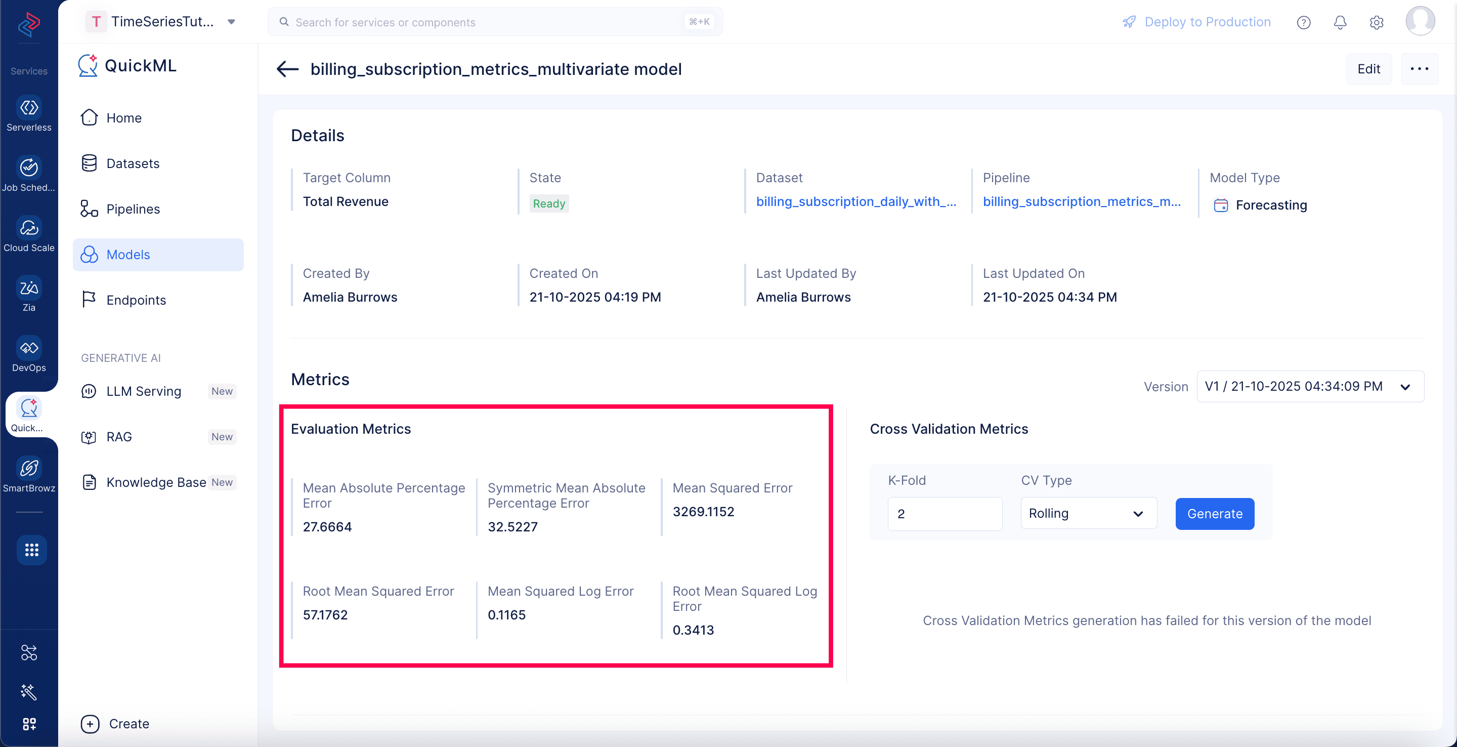
Upon clicking the model hyperlink billing_subscription_metrics_model, the model details page will be opened with necessary information about model details, evaluation metrics, cross validation metrics, and versioning details.

The Model Details page contains the evaluation metrics that help you understand the model performance during the training and validation process, cross-validation metrics, and as well as model versioning details. Model versions are used specifically to track the improvement or degradation of the performance and accuracy of the model upon frequent model training.

As shown in the image below, you can view information about the model on the Model Details page.

Learn more about model evaluation metrics here.