Create an ML pipeline

To build the prediction model, we will use the preprocessed dataset in the ML Pipeline Builder. The initial step in the ML Pipeline Builder involves selecting the target column, which is the column we are trying to predict.

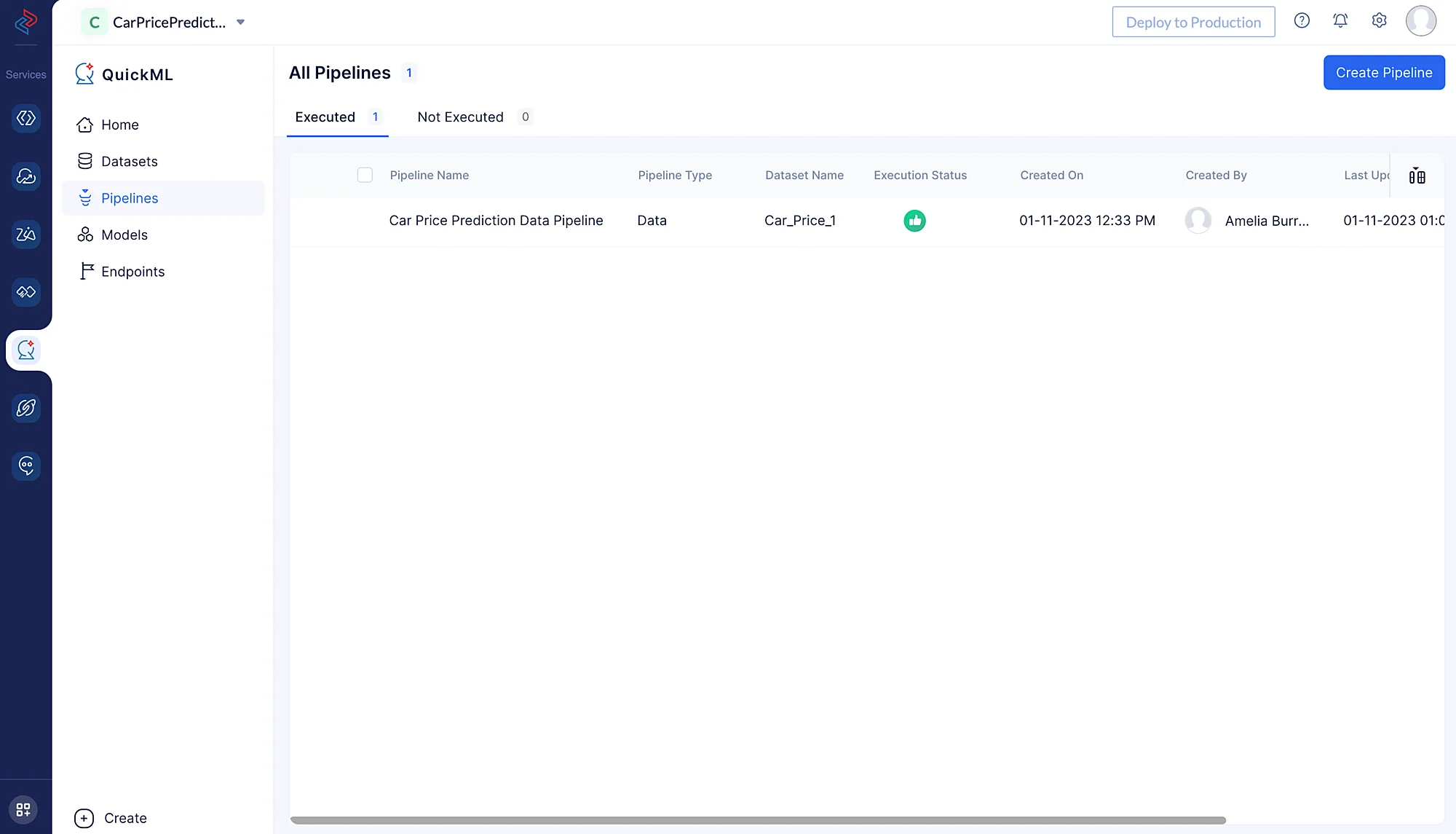
To create an ML pipeline, first navigate to the Pipelines section and click Create Pipeline.

In the pop-up that appears, provide a name (here, we used Car Price Model) for the pipeline and specify the model name. Then, select the appropriate dataset and the column name of the target. In this case, our target is the column named “money”.

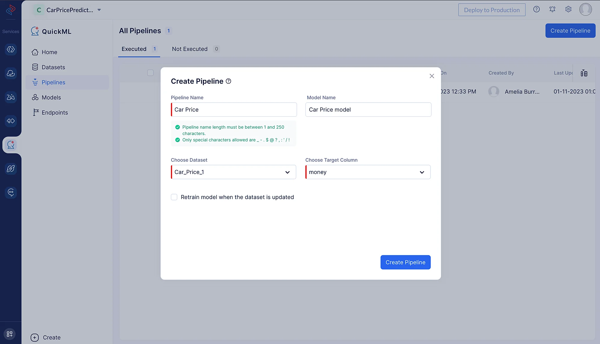
While selecting the dataset, we need to select the source dataset which we chose for building the data pipeline, as the preprocessed data is reflected in the source dataset. In our case, we will be importing the Car_Price_1 dataset, as we have selected this dataset for preprocessing and cleaning the data.

Encoding categorical columns

Encoders are used in various data preprocessing and machine learning tasks to convert categorical or non-numeric data into a numerical format that machine learning algorithms can work with effectively.

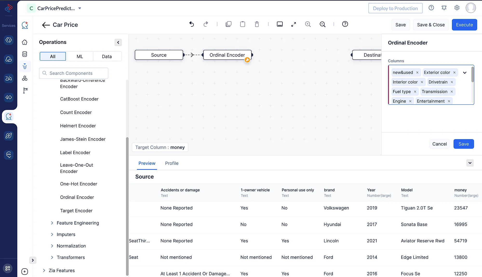
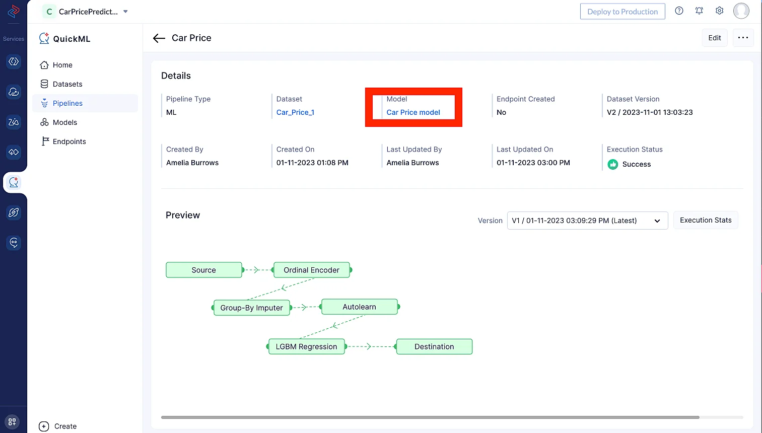
Here, we are using Ordinal Encoding for encoding all the categorical features. It assigns integers to the categories based on their order, making it possible for machine learning algorithms to capture the ordinal nature of the data.

We may use the Ordinal Encoder node from ML Operations > Encoding > Ordinal Encoder in QuickML to turn the category columns into numerical columns. Here, we are converting all categorical columns to numerical format while retaining the columns’ original order and data for model training.

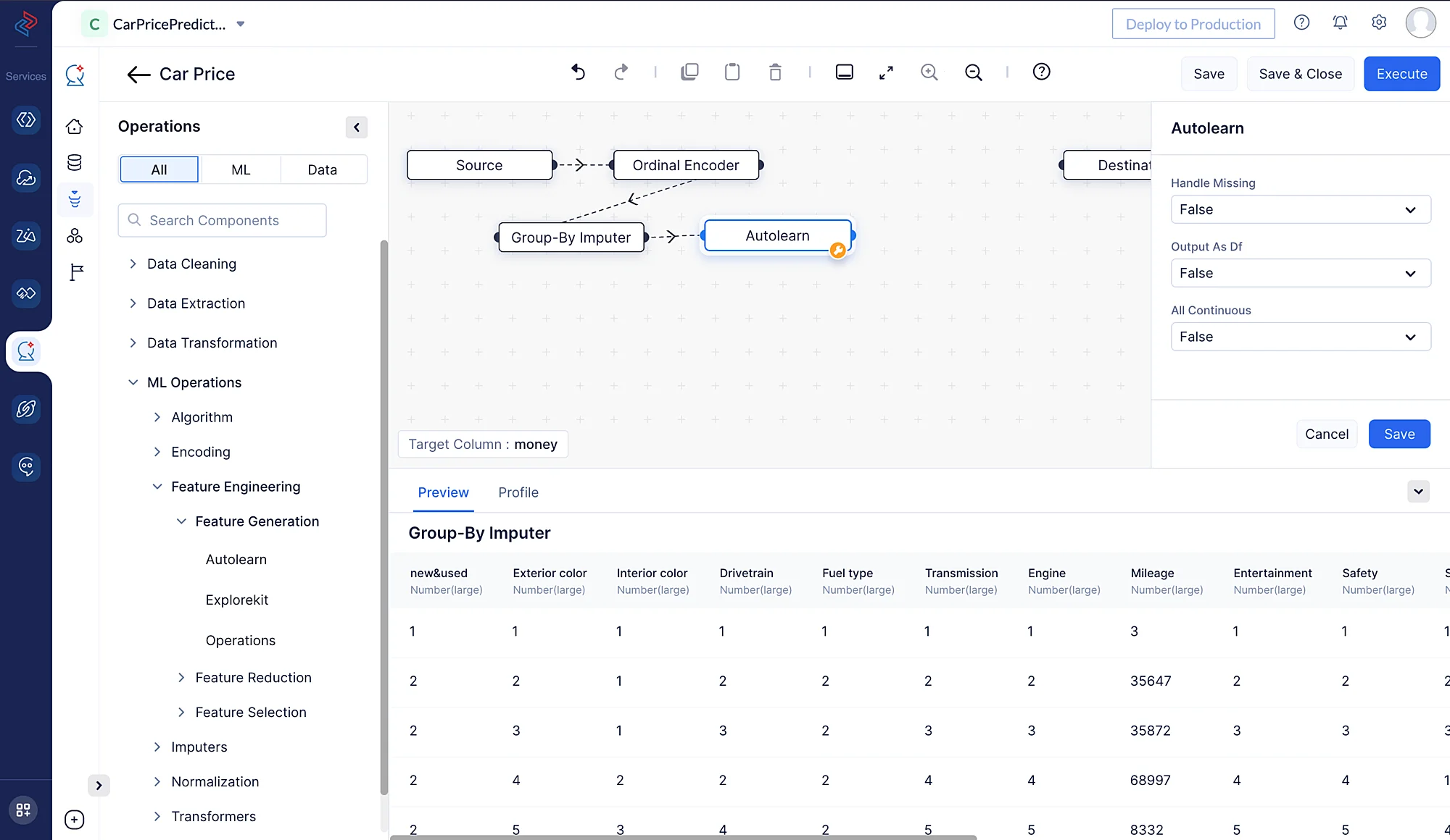
Imputers

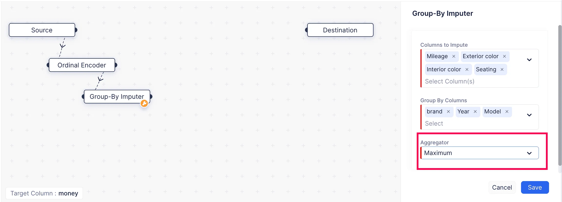
Imputers are used in various fields, such as data analysis, statistics, and machine learning to handle missing or incomplete data. Here, we are using Group By Imputer from ML operations > Imputers > Group-By Imputer for imputing the missing values in the dataset.

Group by Imputing refers to a data imputation technique where missing values are filled based on some grouping or categorization of selected columns. If we can say that a particular column can be imputed by considering another set of column values, we can use this imputation technique.

Here, the columns with missing values are “Mileage”, “Exterior Color”, “Interior Color”, and “Seating”. We have grouped the columns “brand”, “Year”, and “Model” to fill in the missing values.

Feature Engineering

The act of developing new features (variables) from already existing data is referred to as Feature Generation. These additional features can be utilized to enhance the functionality of a machine learning model or to get more insight into the underlying data. A crucial part of the data preprocessing pipeline is feature generation, which can assist transforming raw data into something more suitable for modelling and extract useful information from it.

Here, we have used the “Autolearn” feature generation technique to generate the features. This method generates features from the existing columns. We can select this node from ML Operations > Feature Engineering > Feature Generation > Autolearn.

Selecting algorithm and model fitting

The next step in ML pipeline building is selecting the appropriate algorithm for training the preprocessed data. Here, we’ll use the LightGBM Regressor Algorithm for training the data.

LightGBM (Light Gradient Boosting Machine) is a popular gradient boosting framework used for various machine learning tasks, including regression problems. It is known for its efficiency and speed in training, making it a popular choice for large datasets.

We can quickly construct the LightGBM Regression method in QuickML’s ML Pipeline Builder by dragging and dropping the relevant LightGBM Regression node from ML Operations > Algorithm > Regression > LGBM Regression.

In order to make sure the model is optimized for our particular dataset, we may also adjust the tuning parameters. In our instance, we can just stick with the default settings. When everything is configured, we may save the pipeline for further testing and deployment.

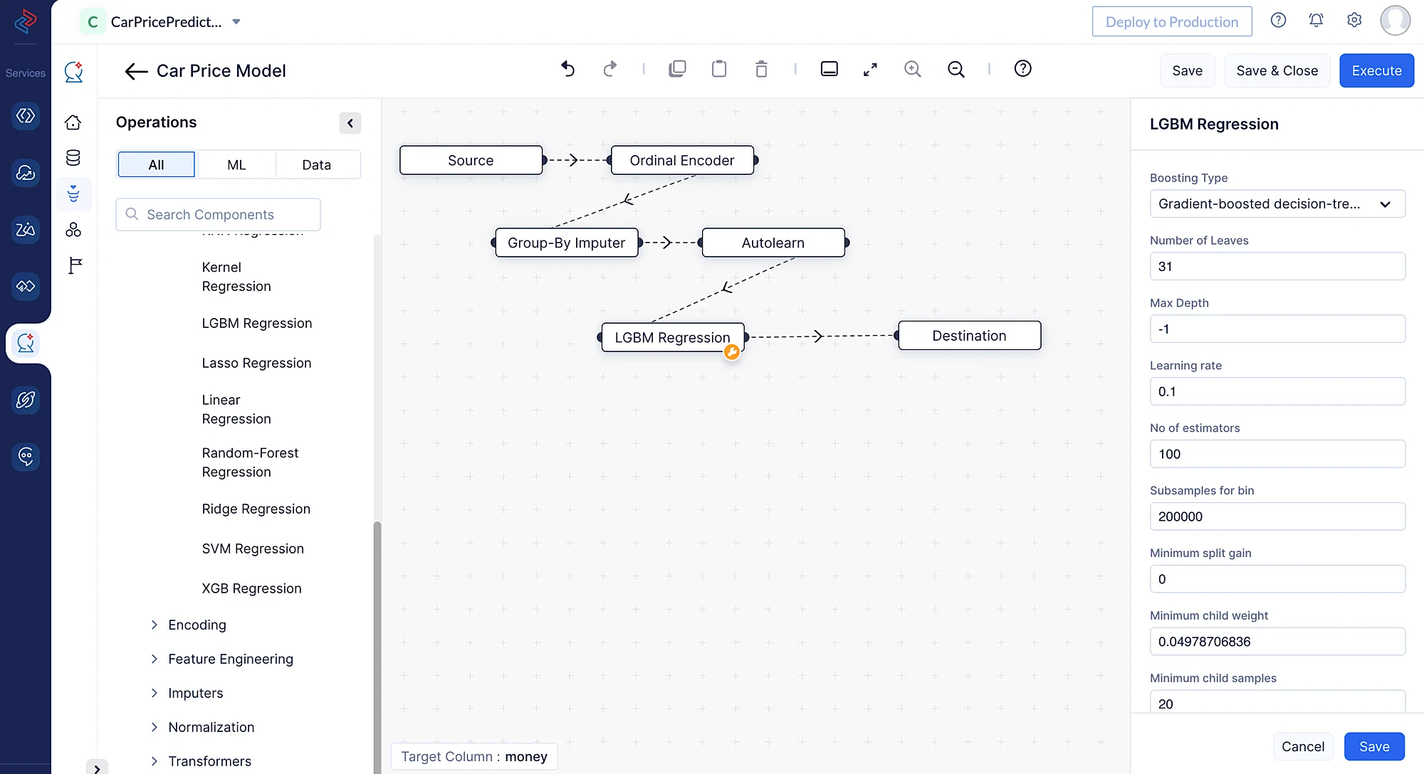
Once we drag-and-drop the algorithm node, its end node will be automatically connected to the destination node. Once the pipeline is saved, you can execute the pipeline by clicking Execute at the top-right corner of the pipeline page.

This will redirect you to the execution page, where you can see the execution of the pipeline.

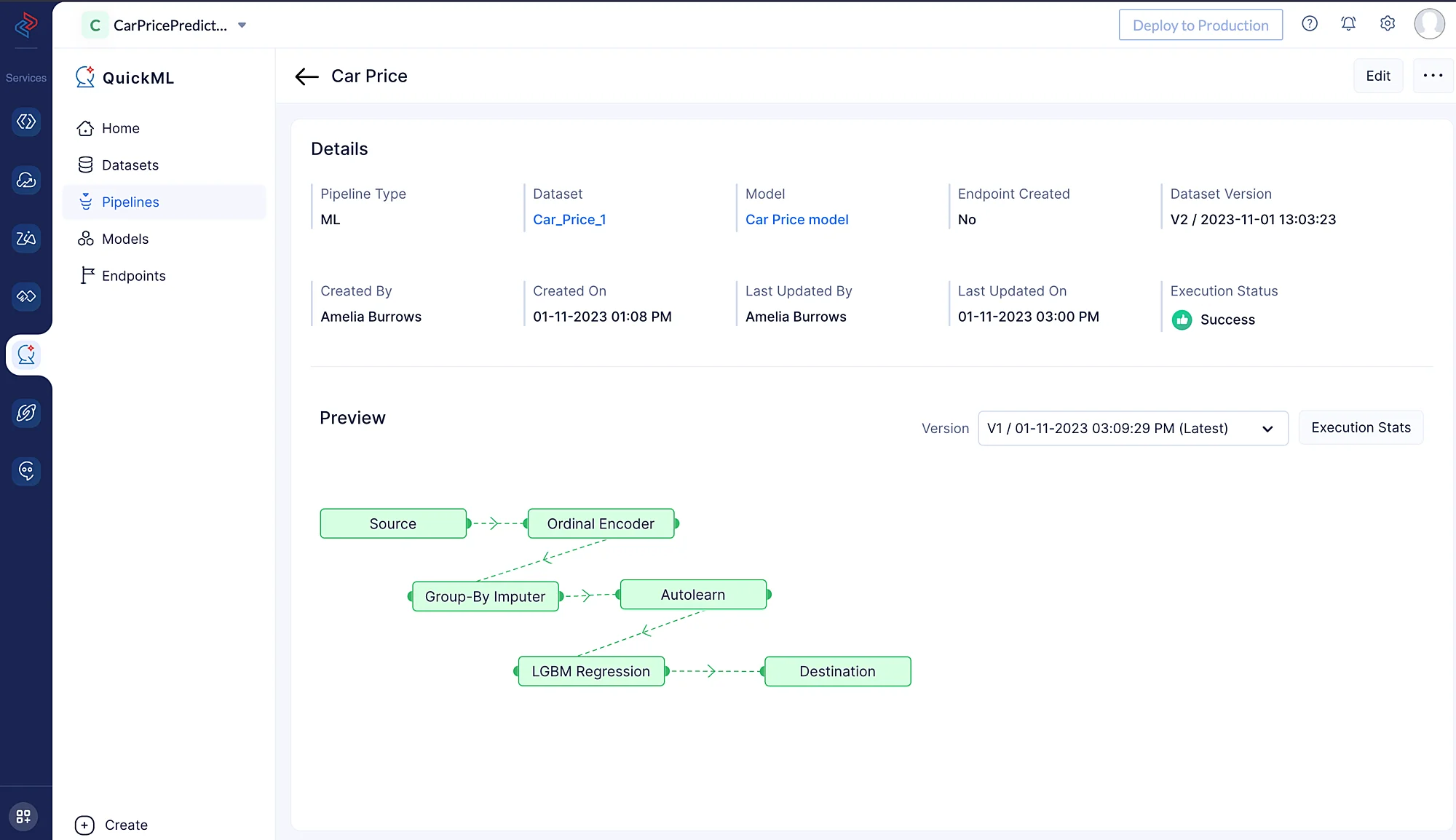
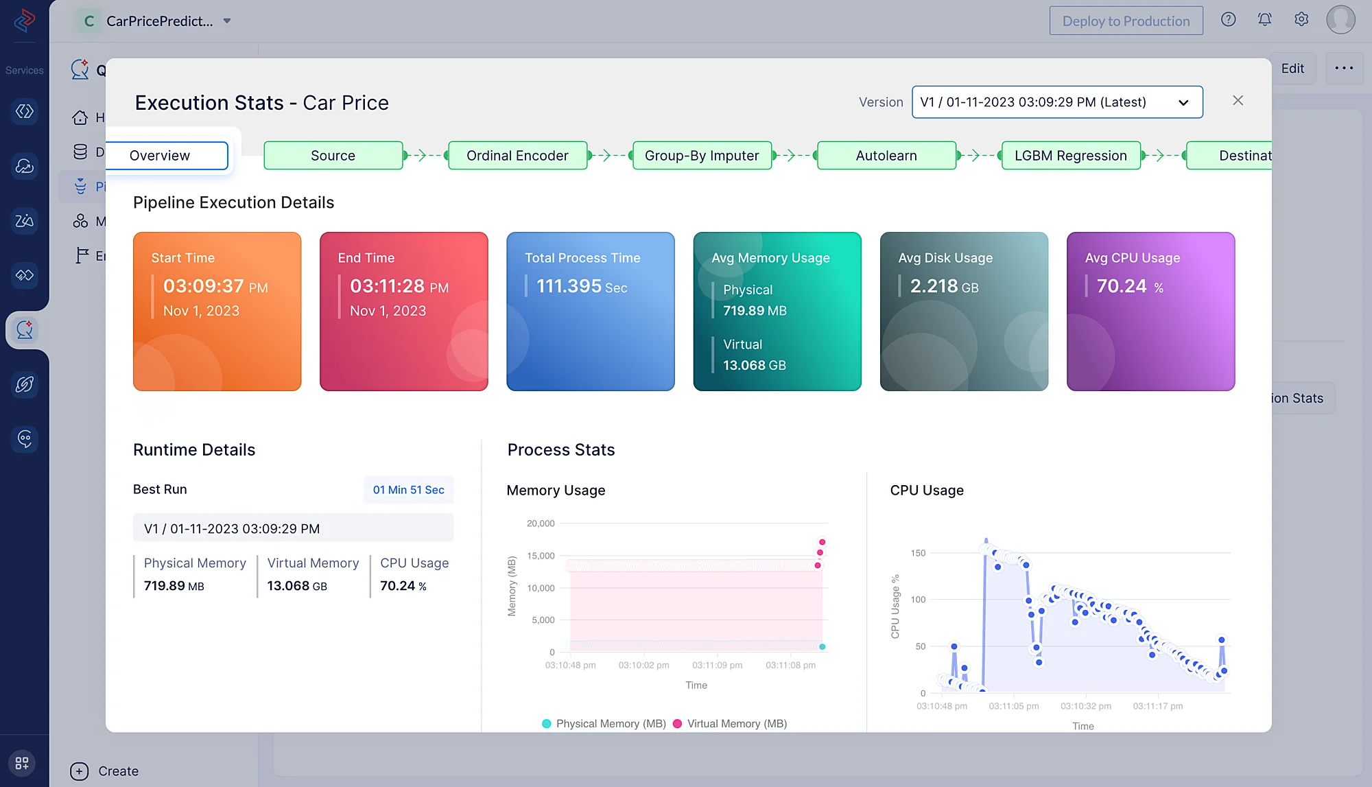
Click Execution Stats to view more details about each stage of the ML pipeline execution in detail.

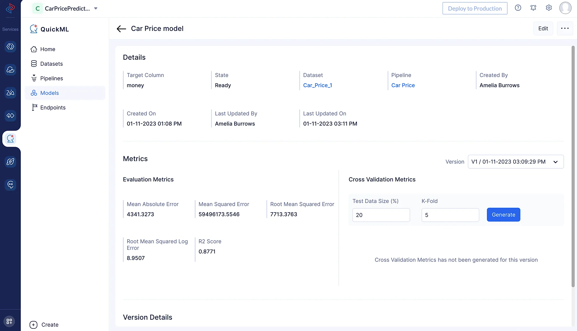
The prediction model is created and can be examined under the Model section (click on Car Price Model model) following the successful execution of the ML workflow.

Metrics below offers useful perceptions into the efficiency and performance of the model while making predictions based on the data.