Prediction Model Generation:

To build the prediction model, we will use the preprocessed dataset in the ML Pipeline Builder. The initial step in the ML Pipeline Builder involves selecting the target column, which is the column we are trying to predict.

In this stage, we will leverage the power of ML Pipeline Builder to construct the machine learning model, enabling us to efficiently predict the target column based on the selected features. The ML Pipeline Builder simplifies the process of model development and provides an intuitive interface for choosing the target column and defining the model’s architecture.

By using ML Pipeline Builder, we can quickly and effectively generate a prediction model tailored to our specific use case, making it an essential tool in the machine learning development process.

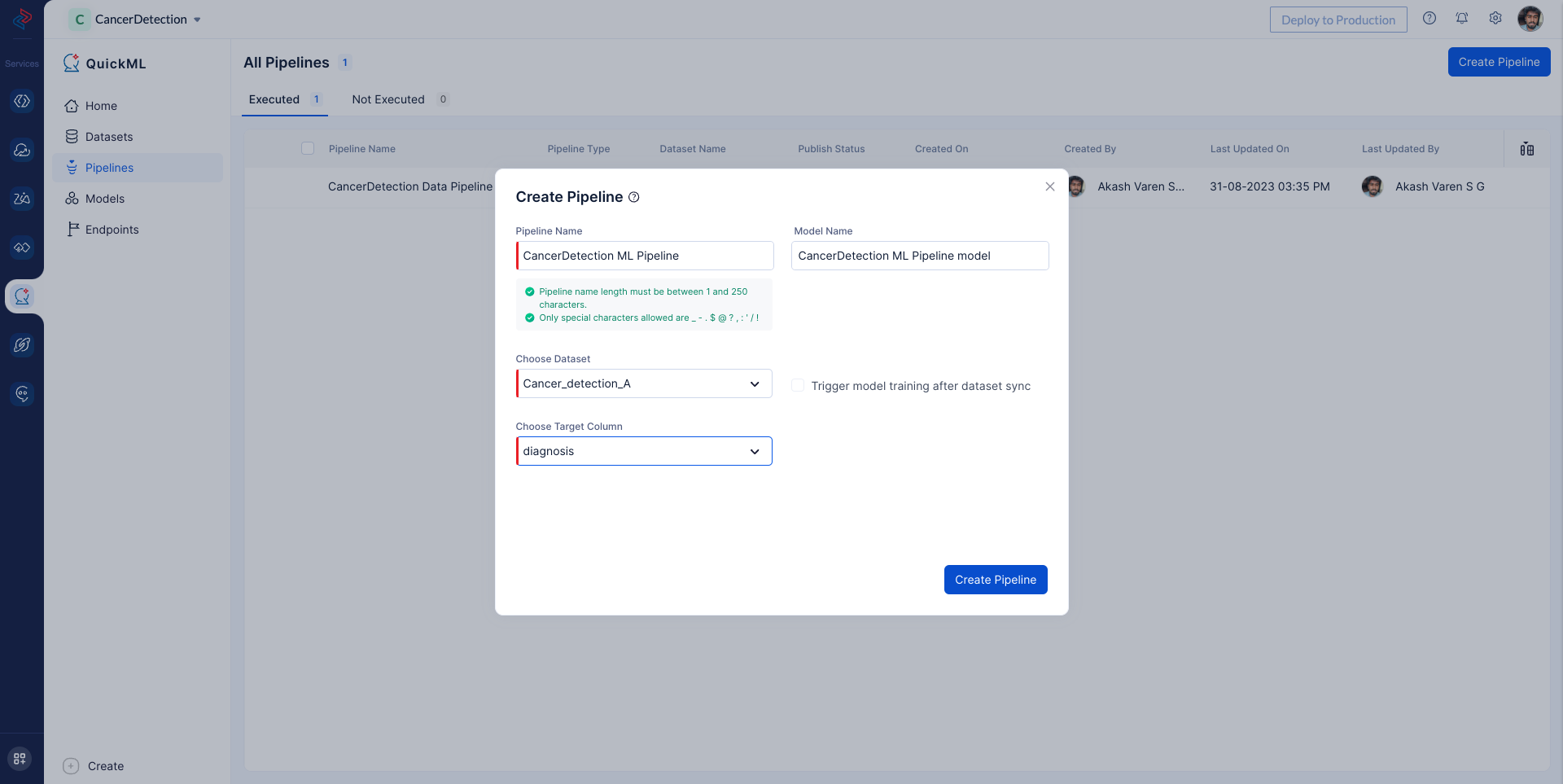
First, navigate to the Pipelines section and click on the Create Pipeline option. Provide a name for the pipeline and specify the model name. Then select the appropriate dataset. In our case, you should choose the Cancer_detection_A dataset that was uploaded previously. Under Target Column, select diagnosis, which is the column our model will predict. The preprocessed dataset will be imported for building the ML pipeline.

Machine Learning Model Creation with and without QuickML:

1. Converting Categorical Data to Numeric using Encoders:

With Python: We will convert all the categorical data in our dataset into numerical format. This process involves using encoding techniques to represent categorical variables as numbers, making them suitable for machine learning algorithms.

    

        
        

            
copy
            

                

            
        
    
    

    

         from sklearn.preprocessing import OrdinalEncoder

# initialize ordinal encoder instance
ordinal_encoder = OrdinalEncoder()
columns_to_encode = ["diagnosis"]

# separate numeric and categorical columns
numeric_dataset = union_dataset.drop(columns=columns_to_encode)
categoric_dataset = union_dataset[columns_to_encode]

# encode the categoric columns
encoded_dataset = pd.DataFrame(
    ordinal_encoder.fit_transform(categoric_dataset),
    columns=columns_to_encode
)

# again concatenate numeric and encoded dataset
preprocessed_dataset = pd.concat(
    [encoded_dataset, numeric_dataset], 
    axis=1
)

         
View more
    

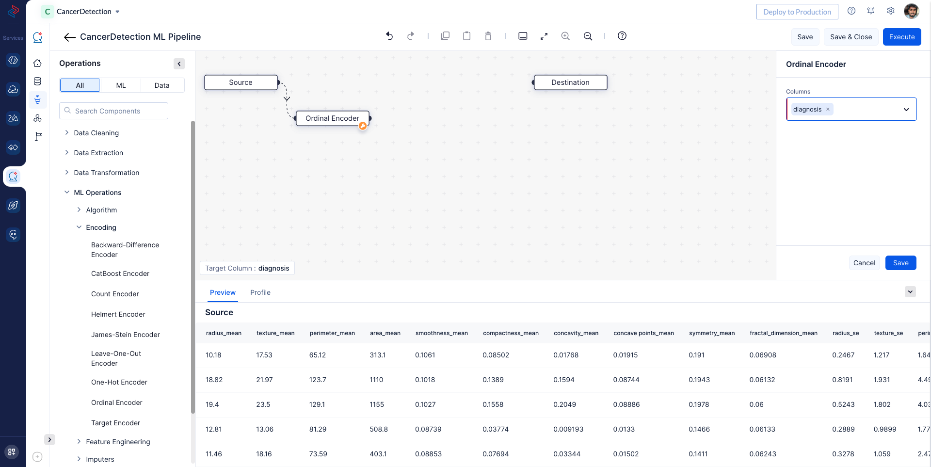
With QuickML: In QuickML’s ML Pipeline Builder, we can convert the “diagnosis” string column into a numerical column using the Ordinal Encoder node. This node allows us to transform the Diagnosis column into a numeric format while maintaining the order and preserving the information for model training.

2. Implementing the Algorithm and Hyperparameter Tuning:

With Python: We will implement the required algorithm to develop our machine learning model. This step involves selecting the appropriate machine learning algorithm based on the nature of our dataset and problem domain.

    

        
        

            
copy
            

                

            
        
    
    

    

         from sklearn.metrics import accuracy_score
from sklearn.linear_model import LogisticRegression

target_name = "diagnosis"

# split the data into features and target
features, target = (
    preprocessed_dataset.drop(columns=target_name), 
    preprocessed_dataset[target_name]
)

# create a logistic regression model
logistic_regression = LogisticRegression(
    penalty='l2',
    tol=0.01831563888,
    C=1.0,
    solver="lbfgs",
    intercept_scaling=1
)

# train a logistic regression model
logistic_regression.fit(features, target)

# predict the features
y_pred = logistic_regression.predict(features)

# compute accuracy score
accuracy_score(y_pred, target)

         
View more
    

Furthermore, we will hyper-tune the model to increase its accuracy and performance. Hyperparameter tuning is a critical process that involves fine-tuning the model’s parameters to optimize its performance and achieve better results.

    

        
        

            
copy
            

                

            
        
    
    

    

         parameters = {
    'penalty': ('l1', 'l2', 'elasticnet'), 
    'C':[1, 2, 5],
    'solver': ('newton-cg', 'lbfgs', 'liblinear', 'sag', 'saga'),
    'max_iter': (150, 160, 200)
}
logistic_regression = LogisticRegression()
clf = GridSearchCV(logistic_regression, parameters)
clf.fit(features, target)
clf.best_params_

         
View more
    

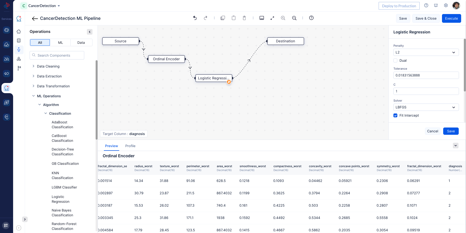
With QuickML: In QuickML’s ML Pipeline Builder, we can easily implement the logistic classification algorithm by dragging and dropping the respective logistic Regression node. Additionally, we can configure the tuning parameters for the model to ensure it is optimized for our specific dataset, in our case we can proceed with default configuration. Once the configuration is complete, we can save the pipeline for further evaluation and deployment.

After completing the node connections, save and Execute the ML Pipeline.

Upon successful execution of the ML Pipeline, the prediction model is created and can be viewed under the Model section. In this section, we can access the details and information about the created model.

Additionally, the accuracy of the generated model can be evaluated and viewed in the metric section of our model details page. This provides valuable insights into the performance and effectiveness of the model in making predictions on the data.

Overall, QuickML’s user-friendly interface and powerful features enable us to effortlessly create, evaluate, and analyze machine learning models, making it a valuable tool for data scientists and developers in various domains.